Verilog-A Functions
| Name | Return type | In types | Implemented? |
| $abstime | real | () | Yes |
| $angle | real | () | No |
| $arandom | integer | (integer,[string]) | Yes |
| $bound_step | none | (real) | Yes |
| $debug | none | ([real/integer/string...]) | Yes |
| $discontinuity | none | ([integer]) | Yes |
| $display | none | ([real/integer/string...]) | Yes |
| $dist_chi_square | integer | (integer,integer) | Yes |
| $dist_erlang | integer | (integer,integer,integer) | Yes |
| $dist_exponential | integer | (integer,integer) | Yes |
| $dist_normal | integer | (integer,integer,integer) | Yes |
| $dist_poisson | integer | (integer,integer) | Yes |
| $dist_t | integer | (integer,integer) | Yes |
| $dist_uniform | integer | (integer,integer,integer) | Yes |
| $error | none | ([string...]) | Yes |
| $fatal | none | (integer, [string...]) | Yes |
| $fclose | none | (integer) | Yes |
| $fdebug | none | (integer, [real/integer/string...]) | Yes |
| $fdisplay | none | (integer, [real/integer/string...]) | Yes |
| $ferror | integer | (integer, string) | Yes |
| $fflush | none | (integer) | Yes |
| $fgets | integer | (string, integer) | Yes |
| $finish | none | ([integer]) | Yes |
| $fmonitor | none | (integer, [real/integer/string...]) | Yes |
| $fopen | integer | (string, [string]) | Yes |
| $fscanf | integer | (integer, string [real/integer/string...]) | Yes |
| $fseek | integer | (integer, integer, integer) | Yes |
| $fstrobe | none | (integer, [real/integer/string...]) | Yes |
| $ftell | integer | (integer) | Yes |
| $fwrite | none | (integer, [real/integer/string...]) | Yes |
| $info | none | ([string...]) | Yes |
| $hflip | real | () | No |
| $limit | real | (access_func,string,real...) | No |
| $mfactor | real | () | Yes |
| $monitor | none | ([real/integer/string...]) | Yes |
| $param_given | integer | identifier | Yes |
| $port_connected | integer | identifier | Yes |
| $random | integer | (integer) | Yes |
| $rdist_chi_square | real | (integer,real, [string]) | Yes |
| $rdist_erlang | real | (integer,real,real, [string]) | Yes |
| $rdist_exponential | real | (integer,real, [string]) | Yes |
| $rdist_normal | real | (integer,real,real, [string]) | Yes |
| $rdist_poisson | real | (integer,real, [string]) | Yes |
| $rdist_t | real | (integer,real, [string]) | Yes |
| $rdist_uniform | real | (integer,real,real,[string]) | Yes |
| $realtime | real | ([real]) | No |
| $rewind | none | (integer) | Yes |
| $sformat | none | (string, string [real/integer/string...]) | Yes |
| $sscanf | integer | (string, string [real/integer/string...]) | Yes |
| $simparam | real | (string,[real]) | Yes |
| $stop | none | ([integer]) | Yes |
| $strobe | none | ([real/integer/string...]) | Yes |
| $swrite | none | (string, string [real/integer/string...]) | Yes |
| $table_model | real | Yes | |
| $temperature | real | () | Yes |
| $vflip | real | () | No |
| $vt | real | ([real] | Yes |
| $write | none | ([real/integer/string...]) | Yes |
| $xposition | real | () | No |
| $yposition | real | () | No |
| above | integer | (real,[real,[real]]) | Yes |
| abs | copies args | (real/int) | Yes |
| absdelay | real | (real, real, [real]) | Yes |
| ac_stim | complex | (string,[real,[real]]) | Yes |
| acos | real | (real) | Yes |
| acosh | real | (real) | Yes |
| analysis | integer | (string,[...]) | Yes |
| asin | real | (real) | Yes |
| asinh | real | (real) | Yes |
| atan | real | (real) | Yes |
| atan2 | real | (real,real) | Yes |
| atanh | real | (real) | Yes |
| ceil | real | (real) | Yes |
| cos | real | (real) | Yes |
| cosh | real | (real) | Yes |
| cross | integer | (real,[integer,[real,[real]]]) | Yes |
| ddt | real | (real,[real/string]) | Yes |
| ddx | real | (real,access_func) | Yes |
| exp | real | (real) | Yes |
| flicker_noise | real | (real,real,[string]) | Yes |
| floor | real | (real) | Yes |
| hypot | real | (real,real) | Yes |
| idt | real | (real,[real,[real,[real/string]]]) | Yes |
| idtmod | real | (real,[real,[real,[real,[real/string]]]]) | Yes |
| laplace_nd | real | (real,real-array,real-array,[real/string]) | Yes |
| laplace_np | real | (real,real-array,real-array,[real/string]) | Yes |
| laplace_zd | real | (real,real-array,real-array,[real/string]) | Yes |
| laplace_zp | real | (real,real-array,real-array,[real/string]) | Yes |
| last_crossing | real | (real,integer) | Yes |
| limexp | real | (real) | Yes |
| ln | real | (real) | Yes |
| log | real | (real) | Yes |
| max | copies args | (real/int,real/int) | Yes |
| min | copies args | (real/int,real/int) | Yes |
| noise_table | real | (real-array,[string]) | No |
| pow | real | (real,real) | Yes |
| sin | real | (real) | Yes |
| sinh | real | (real) | Yes |
| slew | real | (real,[real,[real]]) | Yes |
| sqrt | real | (real) | Yes |
| tan | real | (real) | Yes |
| tanh | real | (real) | Yes |
| timer | integer | (real,[real,[real]]) | Yes |
| transition | real | (real,[real,[real,[real,[real]]]]) | Yes |
| white_noise | real | (real,[string]) | Yes |
| zi_nd | real | (real,real-array,real-array,real,[real,[real]]) | Yes |
| zi_np | real | (real,real-array,real-array,real,[real,[real]]) | Yes |
| zi_zd | real | (real,real-array,real-array,real,[real,[real]]) | Yes |
| zi_zp | real | (real,real-array,real-array,real,[real,[real]]) | Yes |
In this topic:
$abstime
real_time = $abstime ;
In transient analysis, returns the absolute simulation time in seconds. In all other analyses returns zero.
$arandom
value = $arandom[([seed], [type_string])] ;
Where seed is an integer and type_string is a string with value "global" or "instance".
Returns a random number. This has three modes of operation according what if anything is supplied for seed.
Mode 1: no seed
$arandom will return a new random number on each call with the system choosing the seed when random is used for the first time.
Example:
value = $random ;
Mode 2: constant seed
seed may be either a literal constant or a constant expression dependent only on literal constants and parameters. In this mode $arandom will return a new random number on each call using the supplied seed for the starting value. In this mode $arandom will always return the same sequence of values for a given seed.
Example:
parameter seed=23 ;
...
value = $random(seed) ;
Mode 3: initialised integer variable seed
In this mode the seed variable will be updated on each call and a new random number will be generated. The sequence of random numbers will be repeatable given the same initial value for seed.
Example:
integer seed ;
...
@(initial_step)
seed = 23 ;
...
value = $random(seed) ;
In the above, the value of seed will be updated each time random is called.
type_string argument
The type_string argument may be used when $arandom is used in an expression which initialises a parameter. If set to "global", all calls to $arandom with a given seed will return the same random sequence. If set to "instance", the random sequence will vary according to the instance that calls it. All calls for a given instance will return the same sequence.
Note that the use of the type_string argument in a parameter initialisation expression is non-standard and may trigger an error if used with other Verilog-A implementations. LRM 2.4 states that type_string may only be specified in a paramset statement. SIMetrix does not currently implement paramset; these are used for hierarchical construction of Verilog-A modules.
SIMetrix also allows type_string to be used in an analog block expression, but a warning message will be displayed if this is used.
Finally, an "instance" type_string will only have an effect if specified for an instance parameter. Instance parameters are specified using a special attribute. E.g.:
(* type="instance" *)parameter integer ran_num = $arandom(1, "instance") ;
See Also
$bound_step
$bound_step( expression ) ;
Does not return a value.
In transient analysis, instructs simulator to limit the next timestep to the value of expression.
$clog2
$clog2( unsigned_integer_argument ) ;
Returns ceil( log2(argument+1)). It is the minimum number of bits required to represent the integer argument. Note that negative numbers are treated as 32 bit unsigned. E.g. -1 becomes 4294967295 and thus $clog2(-1) = 32.
$debug
$debug( list_of_arguments ) ;
Does not return a value.
$debug is a display function that displays information in the command shell. See $display for a description of its arguments. The $debug function writes to the command shell on every iteration. By contrast, other display functions such as $display only write information when an iteration has converged.
$debug writes an implicit new line character at the end of the text.
See Also
$discontinuity
$discontinuity [ ( constant_expression ) ] ;
Does not return a value.
Currently $discontinuity performs no action.
$display
$display( list_of_arguments ) ;
Does not return a value.
$display displays text in the command shell when the current iteration converges.
The arguments can be any sequence of strings, integers or reals. The function will display these values in the order in which they appear. The values will be output literally except for the interpretation of special characters that may appear in string values. The special characters are backslash ('\') and percent ('%'). '\' is used to output special characters according to the following table:
| \n | Newline character |
| \t | Tab character |
| \\ | Literal \ character |
| \" | " character |
| \ddd | Character specified by the ASCII code of the 1-3 octal digits |
The '%' character must be followed by a character sequence that defines a format specification. In execution, the '%' and the format characters are substituted for the next value in the argument list, formatted according to the string. User's conversant with the 'C' programming language will have seen this method in the printf function. For example, %d specifies that an integer be displayed in decimal format. So, if count has a value of 453, the following:
$display("Count=%d", count) ;
would display:
Count=453
in the command shell.
The following table shows the format codes available:
| %h or %H | Hexadecimal format |
| %d or %D | Decimal format |
| %o or %O | Octal format |
| %b or %B | Binary format |
| %c or %C | ASCII character. E.g a value of 84 would display an uppercase 'T' |
| %m or %M | Display hierarchical name of instance. This does not use one of the subsequent arguments |
| %s or %S | Literal string. Expects a matching string argument |
| %e or %E | Real number format. See Real Number Formats below |
| %f or %F | Real number format. See Real Number Formats below |
| %g or %G | Real number format. See Real Number Formats below |
| %r or %R | Real number format. See Real Number Formats below |
Real Number Formats
Real numbers have their own more complex format codes. These are in the form:
% [flag] [width] [.precision] type
where:
| flag | Characters '-', '+', '0', space or '#'. '-' means left align the result within given width (see width) '+' means always prefix a sign even if positive '0' means prefix with leading zeros '#' forces a decimal point to be always output even if not required |
| width | Specifies the minimum number of characters that will be displayed, padding with spaces or zeros if needed |
| precision | For e and f formats (see below) specifies the number of digits after the decimal point that will be printed. If g or r format is specified, specifies the maximum number of significant digits. Default if omitted is 6. |
| type | e, E, f, F, g, G or r, R e or E: Signed value displayed in exponential format. E.g. 1.23456E3 f or F: Signed value in decimal format. E.g. 1234.56. Result will be very long if value is very large or very small. g or G: Uses either f or e depending on which is most compact for give precision. r or R: displays in engineering units. Uses these scale factors: T, G, M, K, k, m, u, n, p, f, a. |
Notes
The compiler will raise an error if there is a string/numeric mismatch between the format string and supplied arguments. That is if %s found in the format corresponds to an integer or real argument an error will be raised. Conversely if %d or %g etc found in the format string corresponds to a string variable an error will also be raised.
$display("Count=%g", "hello world") ;
No error will result from a real/integer mismatch but a warning will be raised if the format string specifies an integer type but the supplied value is a real.
Note that the type (i.e. integer or real) of literal constants is determined by the way they are written. If a decimal point is included or if exponential or engineering formats are used, the number is real. Otherwise it is an integer. So 11 is an integer, while 11.0 is a real.
See Also
$dist_chi_square
integer_value = $rdist_chi_square( seed, degrees_of_freedom) ;
This function returns a random number with a chi square statistical distribution. seed must be an integer variable initialised with the initial seed value. Each call to the function will update the seed value.
All arguments and return values are integers. In most analog applications the real-valued version $rdist_chi_square is more appropriate.
$dist_erlang
integer_value = $rdist_erlang( seed, k, mean) ;
This function returns a random number with an Erlang statistical distribution. seed must be an integer variable initialised with the initial seed value. Each call to the function will update the seed value.
All arguments and return values are integers. In most analog applications the real-valued version $rdist_erlang is more appropriate.
$dist_exponential
integer_value = $rdist_exponential( seed, mean) ;
This function returns a random number with an exponential statistical distribution. seed must be an integer variable initialised with the initial seed value. Each call to the function will update the seed value.
All arguments and return values are integers. In most analog applications the real-valued version $rdist_exponential is more appropriate.
$dist_normal
integer_value = $rdist_normal( seed, mean, deviation) ;
This function returns a random number with an normal statistical distribution. seed must be an integer variable initialised with the initial seed value. Each call to the function will update the seed value.
All arguments and return values are integers. In most analog applications the real-valued version $rdist_normal is more appropriate.
$dist_poisson
integer_value = $rdist_poisson( seed, mean) ;
This function returns a random number with a poisson statistical distribution. seed must be an integer variable initialised with the initial seed value. Each call to the function will update the seed value.
All arguments and return values are integers. In most analog applications the real-valued version $rdist_poisson is more appropriate.
$dist_t
integer_value = $rdist_t( seed, degrees_of_freedom) ;
This function returns a random number with a T statistical distribution. seed must be an integer variable initialised with the initial seed value. Each call to the function will update the seed value.
All arguments and return values are integers. In most analog applications the real-valued version $rdist_t is more appropriate.
$dist_uniform
integer_value = $rdist_uniform( seed, start, end) ;
This function returns a random number with a uniform statistical distribution. seed must be an integer variable initialised with the initial seed value. Each call to the function will update the seed value.
All arguments and return values are integers. In most analog applications the real-valued version $rdist_uniform is more appropriate.
$error
$error( [list_of_messages]) ;
Does not return a value.
Signals an error condition and terminates the simulation. Unlike $fatal, $error has no effect if called during a rejected iteration. A message stating the time or step along with the reference of the instance that called the function will be written to the list file and displayed in the command shell.
An optional list of message arguments may also be supplied. These use the same format as the $display system task. The messages are displayed in the command shell and the list file.
If $error is called in a multi-step simulation performed using multiple cores, each core will act independently. So only the steps for that particular core will terminate.
A call to $error will set the simulation status to "Error". A subsequent call to the script function GetSimulatorStatus will return 'SimErrors'. (Refer to the Script Reference Manual for details.)
See Also
$fatal
$fatal( finish_code [,list_of_messages]) ;
Does not return a value.
Terminates the simulation immediately. Unlike $error, $fatal will be actioned even if called during an iteration that is rejected.
finish_code can be 0, 1 or 2 as defined in the following table:
| n | Command shell message | List file message | |
| 0 | none | none | |
| 1 | Time and instance ref | Time only | |
| 2 | Time and instance ref | Time and instance ref |
An optional list of message arguments may also be supplied. These use the same format as the $display system task. The messages are displayed in the command shell and the list file.
If $fatal is called in a multi-step simulation performed using multiple cores, each core will act independently. So only the steps for that particular core will terminate.
A call to $fatal will set the simulation status to "Error". A call to the script function GetSimulatorStatus will return 'SimErrors'.
See Also
$fclose
$fclose( file_descriptor ) ;
Does not return a value.
Closes one or more file descriptors opened with $fopen.
See Also
$fdebug
$fdebug( file_descriptor, list_of_arguments ) ;
Does not return a value.
As $debug, but writes to a file or files defined by file_descriptor.
See Also
$fdisplay
$fdisplay( file_descriptor, list_of_arguments ) ;
Does not return a value.
As $display, but writes to a file or files defined by file_descriptor.
See Also
$ferror
integer_value = $ferror( file_descriptor, returned_message_string ) ;
The $ferror function may be called after any other function that operates on a file descriptor to return an error code relating to that function. In addition a descriptive string will be written to the returned_message_string argument.
The Verilog-A language reference manual does not define the codes that this function should return other than 0 meaning "no error". The string written to returned_message_string may be used to display a meaningful message to the user.
if the most recent file operation is a failed call to $fopen, the function will return information about the $fopen call if zero is passed as the file_descriptor.
$fflush
$fflush( file_descriptor) ;
Does not return a value.
Forces the immediate flushing of a file stream. File writes using $fwrite are buffered in memory before being written to disk. This system task forces the buffer to be written out to the file at the end of the current step.
$fgets
integer count = $fgets(string, file_descriptor) ;
Reads a line of text from the file specified by file_descriptor and writes it to the string variable string. The function returns the number of characters read from the file. If an error occurs the return value is zero. Call $ferror to determine the reason for the error.
$finish
$finish [ ( n ) ] | (n, mode)
Does not return a value.
Instructs simulator to finish the analysis. The argument n may take the value of 0, 1 or 2 as shown in the table below:
| n | Command shell message | List file message | |
| 0 | none | none | |
| 1 | Time and instance ref | Time only | |
| 2 | Time and instance ref | Time and instance ref |
If n is omitted, it will default to 1.
$finish is only effective if called during an iteration that converges and is accepted. Any data generated by the converged iteration will be saved as normal.
The mode argument is non-standard and not compatible with other Verilog-A systems. This can have a value of 0 or 1 and determines the behaviour of the function in a multi-step analysis. With a value of 0, or if omitted, the whole simulation will complete and no further steps in the multi-step analysis will be performed. If set to 1, the current step will be terminated but the simulation will continue with the next step.
If $finish is called in a multi-step simulation performed using multiple cores, each core will act independently. So, even with a mode value of 0, only the steps for that particular core will terminate.
A call to $finish is not considered to be an error condition and no error will be flagged. A subsequent call to the script function GetSimulatorStatus will return 'Complete'. (Refer to the Script Reference Manual for details.) To terminate a simulation and flag an error condition, use either $error or $fatal.
The LRM states that $finish should also trigger the final_step event to be executed. SIMetrix does not implement this feature as it is unclear exactly how this should be done. The decision to finish can only be made once the current step has converged as only then are all the values settled to stable values. So it is only at that time that the final_step event code can be executed. To do this would require either one more iteration at the current time step or executing a new time step. Neither makes much sense so we decided not to implement this feature.
If compatibility with other Verilog-A systems is required, we recommend not combining final_step with the $finish system task in the same module.
See Also
$fmonitor
$fmonitor( file_descriptor, list_of_arguments ) ;
Does not return a value.
As $monitor, but writes to a file or files defined by file_descriptor.
$fopen
integer file_descriptor = $fopen( filename [, open_mode] ) ;
This function returns a file descriptor that can be used for any function that writes to or reads from a file.
If the open_mode argument is not supplied, the function operates in multi-channel descriptor mode. Multi-channel descriptors can be used as an argument to functions that write to a file including $fdebug, $fdisplay, $fmonitor, $fstrobe and $fwrite.
There are 31 possible channels each represented by a single bit in the 32 bit returned value. The top (most significant bit) is reserved. The bottom (least siginificant) is used for standard output - i.e. displays to the command shell. Each new call to $fopen will assign the next channel and set the relevant bit. By or'ing together the results from multiple calls to $fopen, it is possible to write to more than one file at a time.
SIMetrix has a special extension to this function providing access to the list file. Use the filename "<listfile>" and the descriptor returned will access it. The following code for example will create a file descriptor that will provide writes to both the list file and a user file:
fd = $fopen( "<listfile>" ) ;
fd = fd | $fopen( "a_text_file.txt") ;
Further, by or'ing with 1 the file descriptor will also write to the command shell.
If the open_mode argument is provided and set to "r", the function will open a file in read mode and return an integer that can be passed to functions that can read data from a file including $fscanf.
if the open_mode argument is provided and set to "w", the function will open a file in write mode and return an integer that can be passed to functions that can write data. This method of creating a write file handle does not suffer from the limit of 31 handles but does not support simultaneous writing of multiple files.
if the open_mode argument is provided and set to "a", the behaviour is the same as "w" except that if the file already exists, new output will be appended to the end of the file.
If the same file is opened for write in two or more instances within the same simulation, an independent file handle will be returned that references a temporary file. When the simulation is complete, the temporary files will be merged with the master file.
The file modes "rb", "wb" and "ab" as described in the LRM are also supported but behave identically to "r", "w" and "a" respectively. On read, the ASCII 13 character ("carriage-return") is always ignored and on write, the CR character is never written out. Currently only text files may be processed using Verilog-A code.
If the specified file cannot be opened, the function returns 0. Note that legitimate file descriptors can be, and usually are, negative. To test whether the file descriptor is valid, be sure to test that it is not equal to zero. Don't test that it is greater than zero.
If the intention is to open a file and keep it open for the duration of an analysis run, the file should be opened in either an initial_step event or an analog intial block. It can then be closed in a final_step event. Note that it is not possible to close a file then reopen it in the same time step.
The file descriptor should be closed with $fclose.
See Also
$fscanf
$fscanf( file_descriptor, format_string, list_of_arguments ) ;
Performs the same function as as $sscanf but instead of reading characters from a string, reads characters from a file defined by the file_descriptor argument. A file_descriptor may be obtained using the $fopen function with the "mode" argument set to "r".
$fseek
integer result $fseek(file_descriptor, offset, op)
Move the file position of the file specified by file_descriptor to the position identified by offset and op. If op is 0, offset is relative to the start of the file. If op is 1, offset is relative to the current position and if op is 2, offset is relative to the end of the file.
The function returns zero if the operation is successful. Otherwise it returns -1. Call $ferror to determine the reason for the error.
Note that if a file is opened in append mode, $fseek is effectively disabled. Append mode does not allow overwriting data already in the file, so the write pointer is always positioned at the end of the file for every write.
See Also
$fstrobe
$fstrobe( file_descriptor, format_string, list_of_arguments ) ;
Does not return a value.
As $strobe, but writes to a file or files defined by file_descriptor. Note that the $strobe and $display functions are identical. For detailed documentation see $display.
See Also
$ftell
integer file_position $ftell(file_descriptor)
Returns the current file position of the file specified by file_descriptor. Returns -1 if an error occurs. Call $ferror to determine the reason for the error.
See Also
$fwrite
$fwrite( file_descriptor, list_of_arguments ) ;
Does not return a value.
As $write, but writes to a file or files defined by file_descriptor. Note that the $write function is identical to $display, except that it does add a new line character. For detailed documentation see $display.
See Also
$info
$info( [list_of_messages]) ;
Does not return a value.
Writes a message to the list file be considered as a low level warning. $info has no effect if called during a rejected iteration.
The message arguments use the same format as the $display system task.
A call to $info will not change the simulation status. A subsequent call to the script function GetSimulatorStatus will return 'Complete'. (Refer to the Script Reference Manual for details).
See Also
$mfactor
real_value = $mfactor ;
$mfactor does not take any arguments.
Returns the scaling factor applied to the instance. The scaling factor may be set using the $mfactor parameter or using a subcircuit multiplier M. If both are used, the final scale factor will be the product of these. Refer to the LRM for more details.
The LRM currently stipulates that compilers should raise an error if $mfactor is used inappropriately. This is not currently implemented and $mfactor may be used for any purpose.
$monitor
$monitor( list_of_arguments ) ;
Does not return a value.
$monitor behaves in a similar manner to $display except that it only outputs a result when there is a change. In other words, the behaviour is the same as $display except that successive repeated messages will not be output.
$monitor writes an implicit new line character at the end of the text.
See Also
$param_given
integer_value = $param_given( parameter_name ) ;
parameter_name must be a parameter defined using the parameter keyword. Returns a non-zero number if parameter_name has been specified in a .MODEL statement or on the instance line where relevant.
$port_connected
integer_value = $port_connected( port_name[ [index_expression] ] ) ;
Returns a non-zero value if the specified port_name is connected externally. If the port is vectored, then index_expression defining the element within the vector must also be specified. No error will be raised if the index supplied is out of range; the function will simply return false (zero).
Currently, this function will only deem a port to be unconnected if no node is specified for it in the instance netlist line. It will return true (non-zero) if a node name is supplied on the netlist line but is not connected to any other component in the netlist. For example, consider a model for a four-terminal BJTwith nodes 'C', 'B', 'E' and 'S' where 'S' is the substrate connection:
Q1 C B E S bjtmodelname
In the above the substrate connection is the node S. In this case $port_connected(S) would return true regardless of whether or not S was connected to anything else. Now consider the three terminal case:
Q1 C B E bjtmodelnameIn this case the substrate connection has been omitted from the netlist line and $port_connected will return false (zero).
$random
integer_value = $random [ (seed) ] ;
Returns a random number. This has three modes of operation according what if anything is supplied for seed.
Mode 1: no seed
$random will return a new random number on each call with the system choosing the seed when random is used for the first time.
Example:
value = $random ;
Mode 2: constant seed
seed may be either a literal constant or a constant expression dependent only on literal constants and parameters. In this mode $random will return a fixed random value which will not update.
Note that this mode of operation is obsolete and may be removed from future releases. To obtain a fixed random value, use $arandom assigned to parameter or localparam. Alternatively assign to a variable in an @initial_step event or analog initial block.
Example:
parameter seed=23 ;
...
value = $random(seed) ;
Mode 3: initialised integer variable seed
In this mode the seed variable will be updated on each call and a new random number will be generated. The sequence of random numbers will thus be repeatable given the same initial value for seed.
Example:
real seed ;
...
@(initial_step)
seed = 23 ;
...
value = $random(seed) ;
In the above, the value of seed will be updated each time random is called.
$rdist_chi_square
real_value = $rdist_chi_square( [ seed ], degrees_of_freedom[, type_string]) ;
Where seed is an integer value and type_string is a string with value "global" or "instance". See $arandom for details of the behaviour of seed and type_string.
This function returns a random number with a chi square statistical distribution.
$rdist_erlang
real_value = $rdist_erlang( [ seed ], k, mean[, type_string]) ;
Where seed is an integer value and type_string is a string with value "global" or "instance". See $arandom for details of the behaviour of seed and type_string.
This function returns a random number with an Erlang statistical distribution.
$rdist_exponential
real_value = $rdist_exponential( [ seed ], mean[, type_string]) ;
Where seed is an integer value and type_string is a string with value "global" or "instance". See $arandom for details of the behaviour of seed and type_string.
This function returns a random number with an exponential statistical distribution.
$rdist_normal
real_value = $rdist_normal( [ seed ], mean, deviation[, type_string]) ;
Where seed is an integer value and type_string is a string with value "global" or "instance". See $arandom for details of the behaviour of seed and type_string.
This function returns a random number with a normal (or Gaussian) statistical distribution.
$rdist_poisson
real_value = $rdist_poisson( [ seed ], mean[, type_string]) ;
Where seed is an integer value and type_string is a string with value "global" or "instance". See $arandom for details of the behaviour of seed and type_string.
This function returns a random number with a poisson statistical distribution.
$rdist_t
real_value = $rdist_t( [ seed ], degrees_of_freedom[, type_string]) ;
Where seed is an integer value and type_string is a string with value "global" or "instance". See $arandom for details of the behaviour of seed and type_string.
This function returns a random number with a T statistical distribution.
$rdist_uniform
real_value = $rdist_uniform( [ seed ], start, end[, type_string]) ;
Where seed is an integer value and type_string is a string with value "global" or "instance". See $arandom for details of the behaviour of seed and type_string.
This function returns a random number with a uniform statistical distribution.
$sformat
$swrite( string_variable, format_string, list_of_arguments ) ;
Does not return a value.
The $sformat function is similar to $swrite with one important difference. $sformat always interprets its second argument, and only its second argument, as a format string.
The remaining arguments to $sformat are processed using any format specifiers in the format_string, until all such format specifiers are used up. If not enough arguments are supplied for the format specifiers or too many are supplied, then a warning will be issued. If the format_string is a literal string constant, i.e. it is not a variable or parameter, then the mismatch detection will be made at compile-time and in this case an error will be raised.
$sscanf
integer_value = $sscanf(string, format_string, list_of_arguments)
$sscanf decodes an input string according to a defined format to write to one or more variables supplied as arguments. The arguments can be any sequence of strings, integers or reals.
The function will read characters from the format string then match the input string according to the following rules:
- A white space character in the format string will match zero or more white space characters in the input string
- A code starting with % in the format string will match a sequence of characters as described in the table below. The % character may followed by an optional sequence of digits representing a maximum width. The sequence of characters up to the maximum width will be read in, decoded then written to the next variable in the argument list
- Any other non-whitespace character in the format string must match exactly each character in the input string
| %d | Integer. Zero or more whitespace characters followed by a sequence of digits with optional '+' or '-' prefix |
| %e, %f or %g | Real. Floating point real number. Zero or more whitespace characters followed by optional '+' or '-' prefix followed by zero or more digits followed by an optional single decimal point followed by zero or more digits optionally followed by 'e' or 'E' followed by an optional '+' or '-' followed by one or more digits. Floating point value is written to variable |
| %r | Real. Floating point real number with engineering suffix. Same as %e, %f or %g followed by an optional single engineering suffix, 'a', 'f', 'p', 'n', 'u', 'm', 'k', 'K', 'M', 'G', 'T'. Each suffix scales the value by the conventional factor. (e.g. 'a': 1e-18, 'm': 1e-3, 'M': 1e6) |
| %s | String. Text string. Zero or more whitespace characters followed by any sequence of characters other than white space |
| %c | Integer. Single character including white space. ASCII code of character is written to corresponding variable |
| %m | String. Does not consume any characters from the input string. Writes the hierarchical reference of the instance to the corresponding string variable |
Any % codes detected in the format that are not in the above table will be ignored. To match a literal % character, use %%.
$sscanf will write to variables that are the correct type only. For example, if %s is detected in the format string, the corresponding input string text will only be written to the corresponding variable if the variable is of type string. If the type is incorrect, no assignment will be made. An exception to this is if the data to be written is an integer and the variable is real. In this instance, the integer value will be written to the real variable.
If there are insufficient variables corresponding to the format string, the input will be consumed but no data will be written. Conversely if there are additional variables with no corresponding codes in the format string, those variables will be ignored.
If the format string is literal (i.e not a variable or model parameter) it will be checked by the compiler at compile time. Any mismatch between the format string and argument list will be detected and reported at that time.
The function will return the number of variables correctly assigned.
$simparam
real_value = $simparam( string [ , default_value ] ) ;
Returns the value of a simulator parameter defined by string. Possible values of string are described below. If an unknown string is supplied, $simparam will return the value of default_value if given. If no default_value value is given, a run-time error will be raised.
| "gdev" | Conductance added in junction GMIN stepping algorithm |
| "gmin" | Value of GMIN options parameter |
| "simulatorSubversion" | Minor version of SIMetrix simulator. E.g. for version 8.00, result will be 0, for 8.30 result will be 30 etc |
| "simulatorVersion" | Major version of SIMetrix simulator. For version 8.30 this will be 8 |
| "sourceScaleFactor" | Scale factor used for sources in source stepping algorithm and pseudo transient analysis algorithm |
| "tnom" | Value of TNOM options parameter |
| "ptaScaleFactor" | Scale factor used for pseudo transient analysis algorithm |
| "option_name" | Any name that may be used in a .OPTIONS statement and which has a real value |
| "iteration" | Iteration number of the solver. This is the local iteration number and is reset to 1 at the start of each time step or sweep step |
| "global_iteration" | Global iteration number is incremented on each iteration and reset at the start of the analysis. In a multi-step run it is reset at the start of each step |
| "startupRamp" | returns value of startup ramp in a transient startup phase. Returns 1.0 normally |
The first six items in the above follow recommended names in the Verilog-A LRM. The remainder are special to SIMetrix.
$simparam$str
real_value = $simparam$str( string ) ;
Similar to $simparam but returns string information. The following strings are supported:
| "analysis_type" | Analysis type one of TRAN, DC, AC, SENS, TF, OP |
| "analysis_name" | Groupname - e.g. tran1, ac2 etc. Note that the group name is not assigned until after the first analysis point has been evaluated. So this string will not work in an analog initial block or initial_step event. |
| "cwd" | Returns the directory where the netlist is located |
| "instance" | Returns the instance name |
| "netlist_path" | Returns the full path of the netlist |
| "module" | Returns the module name |
| "option_name" | Any name that may be used in a .OPTIONS statement and which has a string value |
$simprobe
real_value = $simprobe( instance_name, variable_name [ , default_value ] ) ;
$simprobe returns the value of an output variable from another instance in the circuit. Output variables (also known as readback variables) are listed in the .out file generated when a simulation is run if ".op" or ".options opinfo" is specified in th netlist. For example, BJTs have an output variable called Gm which reports the gain of the device. The following would return the value of Gm for device Q6:
$simprobe( "Q6", "Gm", 0.0 ) ;
In the above call, Q6 is assumed to be a "sibling" instance, that is at the same hierarchical level as the calling device. Prefix with '.' to obtain an absolute reference.
If the instance and or parameter cannot be resolved $simprobe will return the default value supplied. If the default value is omitted, an error will be raised and the simulation will abort.
$simprobe must be used with care. It should not be called in a manner that closes a loop, for example the result of $simprobe must not influence the quantity that it is measuring. Convergence failure is likely if this is done. $simprobe is intended for monitoring and limit testing purposes. So it can be used to report safe operating area violations or it can be used as a probe, but it should not be used as a circuit function.
Including $simprobe in any Verilog-A module affects the timing of the evaluation of that module. This is because $simprobe has to wait until the instances that it is monitoring have been fully evaluated. So $simprobe modules are evaluated later than all others and they are also evaluated in a single non-paralleled thread. This leads the following recommendations:
- $simprobe should not be used to monitor another instance that itself calls $simprobe. The returned value may be inaccurate if this is done.
- $simprobe should not be used in large complex modules that might benefit from parallel processing.
See Also
$stop
$stop [ ( n ) ] ;
The function does not return a value. Pauses simulation after completion of current step and leaves the simulator in the same state as if the user pressed the pause button.
The argument n currently has no effect.
See Also
$strobe
$strobe( list_of_arguments ) ;
Does not return a value.
Identical to the $display function.
See Also
$swrite
$swrite( string_variable, format_string, list_of_arguments ) ;
Does not return a value.
Performs the same function as $fwrite except the results is written to a string variable and not to a file.
For details of the format string and how it is interpreted, see the $display function.
$sx_data_control
$sx_data_control(enable) ;
This function is proprietary to SIMetrix and is not part of the Verilog-A standard.
Enables data output if enable is non-zero. To be useful, regular data output must be disabled. This can be done by setting a data start time that is beyond the analysis stop time, or alternatively by the useDataControl option setting:
.OPTIONS useDataControl
Note that this function can start data output but cannot stop data output.
$table_model
real_value =
$table_model( table_inputs, table_data_source, table_control_string) ;
$table_model implements a multidimensional lookup table. Full details can be found in the language reference manual (LRM) para 9.21 which may be obtained from Verilog-A Language Reference Manual. SIMetrix implements the LRM 2.4 specification in full.
Inputs
The first set of arguments to the function are its inputs, one input for each dimension. So if the table is defined with 2 dimensions, there must be two inputs.
Data Source
The data to define the table is provided after the inputs. This can either be the name of a file in which case the data is read from that file or it can be entered as a series of arrays. There must be at least N+1 arrays where N is the number of dimensions. The first N arrays define values for the corresponding input while the final array defines the output values. There can be more than N+1 arrays with the arrays actually used being defined by the control string. See below for details.
In the LRM and in the following description, data arrays are referred to as columns.
Data Source File Format
The data for the table may be defined in a file. The data in the file is arranged in columns with each value separated by a space or tab. Each row of data must occupy a single line. Comments begin with '#' and continue to the end of that line. They may appear anywhere in the file. Blank lines are ignored. The numbers shall be real or integer.
Control String
The final argument to the function is the control string. This defines a number of options for interpolation, extrapolation and data selection.
The control string is in the form <code>,<code>,...;<out-column>. Each of the <code> strings corresponds to an input column. It consists of up to three characters. The first character may be I, D, 1, 2 or 3 and control the interpolation method as defined in the following table:
| I | Ignore this input column |
| D | Discrete lookup. Use the closest point |
| 1 | Linear interpolation (default) |
| 2 | Quadratic spline interpolation |
| 3 | Cubic spline interpolation |
The interpolation character may be omitted in which case it defaults to linear interpolation.
The second and third characters define the extrapolation method to use when the input variable overruns the table range. The first character defines the behaviour at the lower end and the second character defines the upper end. The letter may be L, C or E as defined below:
| C | Constant extrapolation. The end point value is returned for all input values beyond the table range |
| L | Linear extrapolation. Linear extrapolation is used with a slope consistent with the interpolation method. See notes for details. This is the default |
| E | Error. Raise an error and abort if the converged input value exceeds the table range |
If only one character is provided, it is applied to both ends of the table. If no extrapolation characters are provided, linear extrapolation is used at both ends.
The <out-column> value in the control string defines the column used for the output data. The default is 1 which means the first column encountered after the input data is the output column.
As stated earlier, there must be at least N+1 columns where N is the number of dimensions. The number of dimensions is determined from the number of input variables supplied. There can be more than one column in which case the 'I' character can be used to mark columns that are ignored for input.
It is legal to provide an empty control string, or miss out the argument altogether, in which case all inputs are defined as "1LL" and the output data is at column N+1 where N is the number of dimensions.
| "1LL,3LL" | Assuming 2 dimensions, column 1 defines outer dimension using linear interpolation with linear extrapolation at both ends. Column 2 defines inner dimension using cubic spline interpolation with linear extrapolation at both ends. Output data is in column 3. At least 3 columns must be provided |
| "1LL,3LL;2" | Assuming 2 dimensions, same as above but output data is read from column 4. Column 3 is unused and at least 4 columns must be provided |
| ",3LL;2" | Identical to above. First empty code defaults to "1LL" |
| "EE,3LL;2" | Equivalent to "1EE,3LL;2". As above except outer dimension does not allow excursions outside the data range |
| "2C,1,3,3" | 3 dimensions. Outer dimension uses quadratic spline interpolation with constant extrapolation at both ends. Second dimension uses linear interpolation with linear extrapolation at both ends. Inner dimension uses cubic spline interpolation with linear extrapolation at both ends. Output data is third column after input data, i.e. column 6. |
| 1LC,1LL,I;2 | 2 dimensions. Outer dimension uses first column in data with linear interpolation, linear extrapolation at the lower end and constant extrapolation at the upper end. Inner dimension is defined in the second column and uses linear interpolation and extrapolation. The third data column is ignored and the output data is taken from the second column after the input data, i.e column 5. Column 4 is also ignored. |
Interpolation Methods
Care must be taken when choosing an interpolation method. While the higher order quadratic and cubic spline methods offer a smoother response, they are both capable of exhibiting instability sometimes with disastrous results. This is especially the case when the input data has abrupt changes in slope. The quadratic spline is considerably more prone to this than the cubic spline. It is recommended that a sample test is performed using a DC sweep to check the behaviour.
To see the dangers of specifying spline interpolation, consider the application of fitting the I-V characteristics of a diode to a $table_model function. Below shows such a device modelled using linear interpolation (top) and cubic interpolation (bottom):
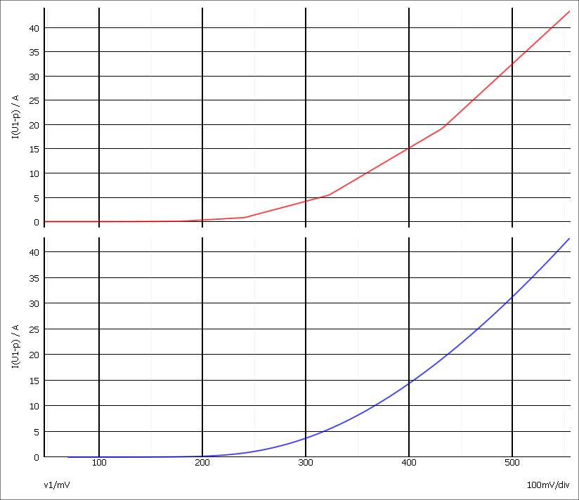 |
Diode table model - high current |
The lower cubic-spline-interpolated curve looks perfectly good and shows a smoother response to the upper linear interpolated response. But now look at the zero crossing:
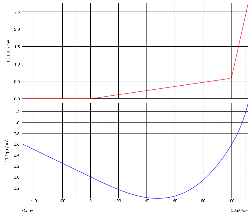 |
Diode table model - low current |
The upper linear curve faithfully follows the entered data points, but the lower cubic- spline-interpolated curve not only goes negative but its slope also reverse sign. This would give completely erroneous results in a simulation. Providing more closely spaced points around the zero crossing can resolve these problems.
The choice of interpolation method may also impact the simulation performance. For the inner most dimension of the table the burden of calculation is small no matter which interpolation technique is chosen. But the choice can affect how quickly the simulation converges and this is circuit dependent. This can only be assessed by experiment.
However, for higher dimensions in a multi-dimension table, there can be a significant performance penalty using anything other than linear or discrete interpolation. For the higher dimensions, the y-values in the lookup table are derived from interpolating a lower dimension and are thus different on each call. This means that the spline coefficients need to be recalculated on every iteration For the spline methods, the entire data set needs to be processed to calculate the coefficients even for just a single segment.
Extrapolation Methods
Three extrapolation options are provided: constant, linear and error. The extrapolation options define how the table function behaves when an input variable exceeds the data range of the table. With constant extrapolation, the end point value is maintained. With linear extrapolation the value follows a straight line with a slope dependent of the interpolation method - see below.
With the error option, the simulation aborts and an error raised if an attempt is made to exceed the input range. Note that the abort only takes place after the iteration has converged and only if the converged result is outside the range. The simulation will not abort if the table input range is exceeded while iterating to convergence but finally converges within range. Linear extrapolation will be selected while iterating to convergence.
The definition of the quadratic and cubic spline interpolators is influenced by the choice of extrapolation. With cubic splines, two constraints, one at each end of the table, need to be set in order to complete the spline definition. If constant extrapolation is selected the constraint is set to be a zero first derivative. If linear extrapolation is set, a zero second derivative is chosen as the constraint and the slope at the end point is chosen as the extrapolation gradient.
For quadratic splines, only a single constraint may be defined. So a zero derivative may be specified at one end but not the other. This leads to a difficulty if both ends are defined with constant extrapolation. The LRM does not define what should be done in this situation. SIMetrix will choose a zero derivative at the lower end, then force continuation of the final point at the upper end. This may lead to a discontinuous slope at the upper end.
$temperature
real_value = $temperature ;
Returns the current simulation temperature in Kelvin.
$vt
real_value = $vt [ ( temperature_expression ) ] ;
Returns the thermal voltage at temperature_expression. If temperature_expression is not supplied, the value at the current simulation temperature will be returned.
The thermal voltage is defined as
\[ \frac{KT}{q} \]
Where, ???MATH???K???MATH??? is boltzmann's constant, ???MATH???T???MATH??? is temperature (defined by temperature_expression) and ???MATH???q???MATH??? is the charge on an electron. The values used for ???MATH???K???MATH??? and ???MATH???q???MATH??? are those that are used for other simulator models and are the best values known at the time the original SPICE program was developed. Since that time the accepted values for ???MATH???K???MATH??? and ???MATH???q???MATH??? have been altered slightly.
- ???MATH???K = 1.3806226\text{e-23}???MATH???
- ???MATH???q = 1.6021918\text{e-19}???MATH???
- ???MATH???K = 1.380649\text{e-23}???MATH???
- ???MATH???q = 1.602176634\text{e-19}???MATH???
$warning
$warning( [list_of_messages]) ;
Does not return a value.
Raises a warning condition. $warning has no effect if called during a rejected iteration. A message stating the time or step along with the reference of the instance that called the function will be written to the list file.
An optional list of message arguments may also be supplied. These use the same format as the $display system task. The messages will be written to the list file.
A call to $warning will set the simulation status to "Warning". A subsequent call to the script function GetSimulatorStatus will return 'Warnings'. (Refer to the Script Reference Manual for details). Warnings may be suppressed using the simulator statement ".options nowarnings".
See Also
$write
$write( list_of_arguments ) ;
Does not return a value.
$write is identical to the $display function except that it does not add a new line character at the end of the text. A new line may be explicitly inserted using the '\n' sequence.
See Also
above
above( expression [,time_tol [,expr_tol [,enable ]]])
above is an event function and may only be used in event expressions. It is identical to the cross event function except that it works in DC analyses and does not have an edge argument.
abs
real_value = abs( x ) ;
Returns the absolute value of x.
absdelay
real_value = absdelay( expression, tdelay [ , maxdelay ] ) ;
Applies a transport delay to an input signal.
| expression | Input signal to delay. |
| tdelay | Delay in seconds. If maxdelay is not supplied, only the value of tdelay at the start of the simulation will be used and subsequent changes will be ignored. Otherwise changes to tdelay will be used as long as they do not exceed maxdelay. |
| maxdelay | Maximum delay permitted. If omitted changes to tdelay will be ignored. See tdelay above. |
In DC analyses, tdelay is ignored and the return value of absdelay is expression. In AC analysis, the signal defined by expression is phase-shifted according to:
\[ \text{output}\left(\omega\right) = \text{input}\left(\omega\right)\exp(-j\omega\cdot\text{tdelay}) \]
In transient analysis, the signal is delayed by an amount equal to the instantaneous value of tdelay as long as it is positive and less than maxdelay. absdelay stores the past history of expression up to maxdelay so that it can retrieve the requested delayed point instantaneously.
absdelay is an analog operator and is subject to Analog Operator Restrictions.
See Also
ac_stim
real_value = ac_stim( [analysis_name_string [ , mag [ , phase ]]] ) ;
Provides a stimulus for AC analysis, essentially identical the AC spec for a standard SPICE voltage source or current source.
| analysis_name_string | Analysis name in which source is to be active. Currently this must be set to "ac" or be omitted altogether. |
| mag | Magnitude of source |
| phase | Phase of source in radians |
acos
real_value = acos( x ) ;
Returns inverse cosine in radians of x. Input range is +/- 1.
acosh
real_value = acosh( x ) ;
Returns the inverse hyperbolic cosine of x. Range is 1.0 to ???MATH???\infty???MATH???.
analysis
integer_value = analysis( analysis_list ) ;
Returns non-zero if the current analysis matches any of the analysis names in the argument list. analysis_list is a list of strings as defined in the following table.
| "static" | Any analysis that solves a DC operating point. This includes the operating point analyses carried before other analyses such as transient. It also includes DC sweep |
| "tran" | Transient analysis. Includes the transient analysis used for pseudo transient analysis |
| "ac" | AC analysis |
| "dc" | DC sweep |
| "noise" | Noise analysis not including real time noise |
| "tf" | Transfer fumction analysis |
| "pz" | Pole zero analysis |
| "sens" | Sensitivity analysis |
| "ic" | The dc operating point analysis that precedes a transient analysis |
| "smallsig" | Any small signal analysis: AC, noise and TF |
| "rtn" | Real-time noise analysis |
| "pta" | Pseudo transient analysis |
asin
real_value = asin (x ) ;
Returns the inverse sine in radians of x. Range is +/- 1.0.
asinh
real_value = asinh( x ) ;
Returns the inverse hyperbolic sine of x. Range is ???MATH???-\infty???MATH??? to ???MATH???+\infty???MATH???.
atan
real_value = atan( x ) ;
Returns the inverse tangent in radians of x. Range is ???MATH???-\infty???MATH??? to ???MATH???+\infty???MATH???.
atan2
real_value = atan2( x, y ) ;
Returns the inverse tangent in radians of x/y. The function will return a meaningful value when y is zero.
atanh
real_value = atanh( x ) ;
Returns the inverse hyperbolic tangent of x. Range is +/- 1.0.
ceil
real_value = ceil( x ) ;
Returns the next integer value greater than x.
cos
real_value = cos( x ) ;
Returns the cosine of x expressed in radians. Range is ???MATH???-\infty???MATH??? to ???MATH???+\infty???MATH???.
cosh
real_value = cosh( x ) ;
Returns the hyperbolic cosine of x. Range is approx -709 to +709.
cross
cross( expression [,edge [,time_tol [,expr_tol [,enable ]]]])
cross is an event function and may only be used in event expressions.
| expression | expression to test. The event is triggered when the expression crosses zero. |
| edge | 0, +1 or -1 to indicate edge. +1 means the event will only occur when expr is rising, -1 means it will only occur while falling and 0 means it will occur on either edge. Default=0 if omitted. |
| time_tol | Time tolerance for detection of zero crossing. Unless the input is moving in an exact linear fashion, it is not possible for the simulator to predict the precise location of the crossing point. But it can make an estimate and then cut or extend the time step to hit it within a defined tolerance. time_tol defines the time tolerance for this estimate. The event will be triggered when the difference between the current time step and the estimated crossing point is less than time_tol. See diagram below for an illustration of the meaning of this parameter. |
| expr_tol | Similar to time_tol but instead defines the tolerance on the input expression. See figure below. |
| enable | if zero, the event function will be disabled |
if neither time_tol nor expr_tol are defined or are both set to zero, a default time_tol value will be chosen.
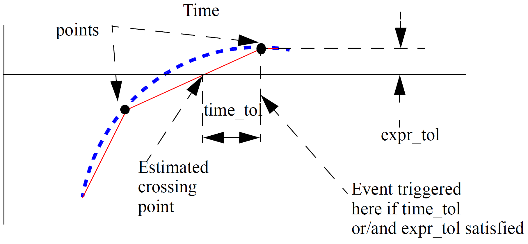 |
Cross Event Function Behaviour |
cross stores state information in the same way as an analog operator. It is therefore subject to Analog Operator Restrictions.
See Also
ddt
real_value = ddt( expression ) ;
Returns the time derivative of expression:
\[ \frac{d}{dt}\text{expression} \]
In DC analyses, ddt returns zero. In AC analysis, the function is defined by the relation:
\[ \text{output}\left(\omega\right) = input\left(\omega\right)\cdot j\omega \]
ddt is an analog operator and is subject to Analog Operator Restrictions.
See Also
ddx
real_value = ddx( expression, unknown_variable) ;
Performs symbolic differentiation on expression with respect to unknown_variable, which must be defined in terms of an access function in one of the following forms:
potential_access_identifier( net_or_port_scalar_expression )OR
flow_access_identifer( branch_identifier )
A potential_access_identifier is defined in the discipline declarations and is usually 'V' for the electrical discipline. Similarly, the flow_access_identifier is usually 'I' for the electrical discipline.
net_or_port_scalar_expression can be a module port node or an internal node.
branch_identifier can be a branch defined with the branch keyword or an unnamed branch specifying the nodes connected to the branch.
exp
real_value = exp( x ) ;
Returns the exponential of x. Range is ???MATH???-\infty???MATH??? to about 709.
See Also
flicker_noise
real_value = flicker_noise( power, exp [, name]) ;
flicker_noise is only active in small-signal noise analysis and real-time noise analysis; in other analysis modes it returns zero. It creates a noisy signal with a power of power at 1Hz which varies in proportion to ???MATH???1/f^{\text{exp}}???MATH???.
name may be used to combine noise sources in the output report and vectors. Noise sources with the same name in the same instance will be combined together.
In real-time noise analysis flicker_noise simply returns a random number whose statistical distribution satisfies the characteistic of ???MATH???1/f???MATH??? noise. In small signal analysis flicker_noise defines a ???MATH???1/f???MATH??? noise source that may be propagated to any output node.
See Also
hypot
real_value = hypot( x, y ) ;
Returns ???MATH???\sqrt{x^2 + y^2}???MATH???.
idt
real_value = idt( expression [, initial_condition [, assert [, abstol]] ] ) ;
Returns the time integral of expression.
initial_condition if supplied, sets the value of the function for DC analyses including the dc operating point that precedes other analyses.
If initial_condition is not supplied, idt must exist inside a closed feedback loop. With no initial condition the DC gain of idt is infinite; by putting the function inside a loop, the simulator can maintain the input at zero providing a finite output. A singular matrix error will result otherwise.
If assert is non-zero, the integrator is reset and the return value is the value of initial_condition. Care should be taken when using assert as it can result in discontinuous behaviour leading to convergence problems.
abstol is accepted but currently is not functional.
idt is an analog operator and is subject to Analog Operator Restrictions.
See Also
idtmod
real_value = idtmod( expression [, ic [, modulus [, offset [, abstol]]] ] ) ;
Returns the time integral of expression.
ic if supplied, sets the value of the function for DC analyses including the dc operating point that precedes other analyses.
If ic is not supplied, idt must exist inside a closed feedback loop. With no initial condition the DC gain of idt is infinite; by putting the function inside a loop, the simulator can maintain the input at zero providing a finite output. A singular matrix error will result otherwise.
modulus and offset: modulus is an expression that must evaluate to a positive value. If not present, idtmod() behaves like idt(). If present, idtmod() returns k where offset <= k < modulus. ???MATH???$\int x(t)dt + ic = n.modulus + k???MATH???$ where n is an integer and ic is the initial condition. offset is zero if not provided.
idtmod is an analog operator and is subject to Analog Operator Restrictions.
See Also
laplace_nd
real_value = laplace_nd(expr, num_coeffs, den_coeffs [, $\epsilon$]) ;
| expr | Input expression. |
| num_coeffs | Numerator coefficients. This can be entered as an array variable or as an array initialiser. An array initialiser is a sequence of comma separated values enclosed with '{' and '}'. E.g: { 1.0, 2.3, 3.4, 4.5}. The values do not need to be constants. |
| den_coeffs | Denominator coefficients in the same format as the numerator - see above. |
| ???MATH???\epsilon???MATH??? | Tolerance parameter currently unused. |
The laplace_nd analog operator implements a Laplace transfer function. This is in the form:
\[ H(s) = \frac{n_0 + n_1\cdot s + n_s\cdot s^2 + ... + n_m\cdot s^m}{d_0 + d_1\cdot s + d_2\cdot s^2 + ... + d_m\cdot s^m} \]
where ???MATH???d_0, d_1, d_2, ..., dm???MATH??? are the denominator coefficients and ???MATH???n_0, n_1, n_2, ..., n_m???MATH??? are the numerator coefficients and the order is ???MATH???m???MATH???.
If the constant term on the denominator ( ???MATH???d_0???MATH??? in equation above) is zero, the laplace function must exist inside a closed feedback loop. With a zero denominator, the DC gain is infinite; by putting the function inside a loop, the simulator can maintain the input at zero providing a finite output. A singular matrix error will result otherwise.
laplace_nd is an analog operator and is subject to Analog Operator Restrictions.
See Also
laplace_np
real_value = laplace_np(expr, num_coeffs, poles [, $\epsilon$]) ;
| expr | Input expression |
| zeros | Zeros. See laplace_zp for details. |
| den_coeffs | Denominator coefficients. See laplace_nd for details. |
| ???MATH???\epsilon???MATH??? | Tolerance parameter currently unused |
laplace_np is an analog operator and is subject to Analog Operator Restrictions.
See Also
laplace_zd
real_value = laplace_zd(expr, zeros, den_coeffs [, $\epsilon$]) ;
| expr | Input expression. |
| zeros | Zeros. See laplace_zp for details. |
| den_coeffs | Denominator coefficients. See laplace_nd for details. |
| ???MATH???\epsilon???MATH??? | Tolerance parameter currently unused. |
laplace_zd is an analog operator and is subject to Analog Operator Restrictions.
See Also
laplace_zp
real_value = laplace_zp(expr, zeros, poles [, $\epsilon$]) ;
| expr | Input expression. |
| zeros | Array of pairs of real numbers representing the zeros of the Laplace transform. Each pair consists of a real part and an imaginary part with the real part first. Each zero introduces a product term on the numerator in the form: \[ 1-\frac{s}{\textit{re} + j\cdot \textit{im}} \] where re is the real part and im imaginary part. If a zero is complex (i.e. the imaginary part is non-zero) then its complex conjugate must also be present. If both real and imaginary parts are zero then the zero becomes just s. The values can be entered as an array variable or as an array initialiser. An array initialiser is a sequence of comma separated values enclosed with '{' and '}'. E.g: {1.0, 2.3, 3.4, 4.5}. The values do not need to be constants. |
| poles | Array of pairs of real numbers representing the poles of the Laplace transform. Each pair consists of a real part and an imaginary part with the real part first. Each pole introduces a product term on the denominatr in the form: \[ 1-\frac{s}{\textit{re} + j\cdot \textit{im}} \] where re is the real part and im imaginary part. If a pole is complex (i.e. the imaginary part is non-zero) then its conjugate must also be present. If both real and imaginary parts are zero then the pole becomes just s. The values can be entered as an array variable or as an array initialiser. An array initialiser is a sequence of comma separated values enclosed with '{' and '}'. E.g: {1.0, 2.3, 3.4, 4.5}. The values do not need to be constants. |
| ???MATH???\epsilon???MATH??? | Tolerance parameter currently unused. |
laplace_zp is an analog operator and is subject to Analog Operator Restrictions.
See Also
last_crossing
real_value = last_crossing( expression, direction ) ;
last_crossing returns the time in seconds when expression last crossed zero. First order interpolation is used to estimate the time of the crossing. direction controls the direction of the crossing. If +1 then the most recent positive transition is returned. If -1, the most recent negative transition and if zero the most recent in either direction is returned.
last_crossing returns a negative number if expression has not crossed zero since the start of the simulation. SIMetrix Verilog-A last_crossing implementation also returns a negative number for DC analyses but this is not defined in the standard.
last_crossing is an analog operator and is subject to Analog Operator Restrictions.
limexp
real_value = limexp( x ) ;
Returns the exponential of x. limexp limits its change in output from iteration to iteration in order to improve convergence. In situations where its return value is not the true exponential of x it will force further iterations. The iteration will only be accepted when the result is the true value of exp(x). Thus, limexp can be seen as a direct replacement for exp but with improved convergence. But note that limexp is an analog operator and is therefore subject to Analog Operator Restrictions.
See Also
ln
real_value = ln( x ) ;
Returns the natural logarithm of x. Range is 0.0 to ???MATH???\infty???MATH???.
log
real_value = log( x ) ;
Returns the logarithm to base 10 of x. Range is 0.0 to ???MATH???\infty???MATH???.
max
real_value = max( x, y ) ;
Returns x or y whichever is larger. Equivalent to ( x>y ? x : y )
min
real_value = min( x, y ) ;
Returns x or y whichever is smaller. Equivalent to ( x<y ? x : y )
pow
real_value = pow( x, y ) ;
Returns ???MATH???x^y???MATH???. if x is less than zero, y must be an integer. If ???MATH???x=0???MATH???, y must be greater than zero.
sin
real_value = sin( x ) ;
Returns the sine of x given in radians. Range ???MATH???-\infty???MATH??? to ???MATH???\infty???MATH???.
sinh
real_value = sinh( x ) ;
Returns the hyperbolic sine of x. Range is approx -709 to +709.
slew
real_value = slew( expression [, slew_pos [, slew_neg]] ) ;
Implements a slew rate limiter. slew_pos is expected to be positive and slew_neg is expected to be negative. If slew_neg is not specified or greater than or equal to zero, it assumes a value of -slew_pos. If neither slew_pos or slew_neg is present, expression is passed through to value unchanged.
slew limits the positive and negative rate of change of its return value to slew_pos and slew_neg respectively.
slew is an analog operator and is subject to Analog Operator Restrictions.
See Also
sqrt
real_value = sqrt( x ) ;
Returns the square root of x. Range is 0 to ???MATH???\infty???MATH???. Although valid, ???MATH???x=0???MATH??? should be avoided and if possible code included to prevent ???MATH???x=0???MATH???. This is because the first derivative of sqrt at zero is infinite and convergence at this value can be problematic.
tan
real_value = tan( x ) ;
Returns the tangent of x given in radians. Range is ???MATH???-\infty???MATH??? to ???MATH???\infty???MATH???.
tanh
real_value = tanh( x ) ;
Returns the hyperbolic tangent of x. Range is ???MATH???-\infty???MATH??? to ???MATH???\infty???MATH???.
timer
timer( time [, period [, time_tol [, enable]]])
timer is an event function and may only be used in an event statement in the form:
@(timer(...))
statement ;
statement is executed when the event is triggered.
timer sets a future event to occur at a specified time either just once or repeating at a specified period.
The event is first scheduled at time. If period is specified and is greater then zero, subsequent events will also be scheduled at time + n*period where n is a positive integer.
Usually the specified event will be scheduled at exactly the time specified. However, the analog simulator will not allow time points to be forced too close together as this can lead to numerical problems as well as unnecessarily long simulation times. For this reason, the simulator may schedule the event slightly later than specified if the time point is too close to an existing time point, perhaps set by another device. The time_tol argument controls the tolerance of the event time. The simulator will always schedule the event so that it is within time_tol of the requested time. If time_tol is not specified the event will be scheduled after the requested time but not more than the amount specified by the MINBREAK simulation parameter.
if enable is zero, the event function will be disabled.
See Also
transition
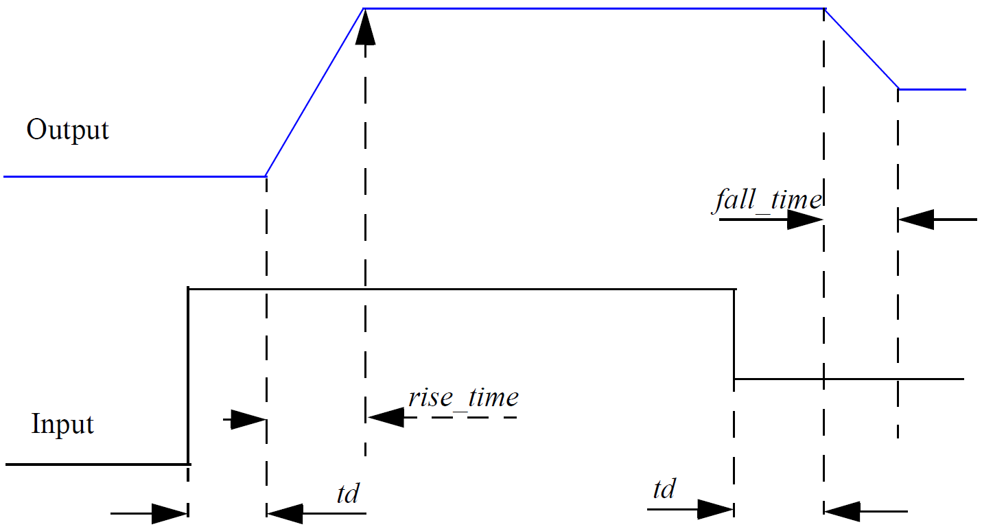
real_value = transition(expr[, td[, rise_time[, fall_time [, time_tol]]]]);
The transition analog operator converts the discrete input value to a continuous output value using specified rise and fall times.
Its arguments are:
| expr | Input expression. |
| td | Delay time. This is a transport or stored delay. That is, all changes will be faithfully reproduced at the output after the specified delay time, even if the input changes more than once during the delay period. This is in contrast to inertial delay which swallows activity that has a shorter duration than the delay. Default=0. |
| rise_time | Rise time of output in response to change in input. |
| fall_time | Fall time of output in response to change in input. |
| time_tol | Currently ignored. |
If fall_time is omitted and rise_time is specified, the fall_time will default to rise_time. If neither is specified or are set to zero, a minimum but non-zero time rise/fall time is used. This is set to the value of MINBREAK which is the minimum break point value. Refer .OPTIONS in the Simulator Reference Manual/Command Reference/.OPTIONS for details of MINBREAK.
The transition analog operator should not be used for continuously changing input values; use the slew or absdelay analog operators instead.
transition is an analog operator and is subject to Analog Operator Restrictions.
See Also
white_noise
real_value = white_noise( power [, name]) ;
white_noise is only active in small-signal noise analysis and real-time noise analysis; in other analysis modes it returns zero. It creates a noisy signal with a power of power and a flat frequency distribution.
name may be used to combine noise sources in the output report and vectors for small-signal noise analysis. name is ignored with real-time noise analysis. Noise sources with the same name in the same instance will be combined together.
In real-time noise analysis white_noise simply returns a random number whose statistical distribution satisfies the characteristic of Gaussian noise. In small signal analysis white_noise defines a noise source that may be propagated to any output node.
See Also
zi_nd
real_value = zi_nd(expr,numerator,denominator,interval,[transition,[delay]]) ;
The zi_nd function implements a linear discrete-time filter defined by z-transform coefficients for both numerator and denominator. Its arguments are:
| expr | Input expression |
| numerator | Array of numerator coefficients in increasing order |
| denominator | Array of denominator coefficients in increasing order |
| interval | Sampling interval in seconds |
| transition | rise and fall time of output at each step |
| delay | Delay in seconds |
The function implements the z-transform:
???MATH???\frac{ \displaystyle \sum^{M-1}_{k=0}n_k z^{-k}}{ \displaystyle \sum^{N-1}_{k=0}d_k z^{-k} }???MATH???
where ???MATH???n_k???MATH??? is the ???MATH???k^{th}???MATH??? numerator coefficient and ???MATH???d_k???MATH??? is the ???MATH???k^{th}???MATH??? denominator coefficient.
The numerator and denominator coefficients may be passed to the function either as array parameters or variables or directly as array initialisers. An array initialiser is a sequence of comma separated values enclosed with '{' and '}'. E.g: { 1.0, 2.3, 3.4, 4.5}. The values do not need to be constants. If they are non-constant, the value at the start of the simulation will be used
If transition is omitted, a default minimum time is used. If it is set to zero, the transition time will be uncontrolled; in this case the result of this function should be further filtered to avoid convergence issues. The Verilog-A LRM does not allow a z-transform filter to be directly assigned to a branch if a transition time of zero is set. Currently, SIMetrix does not enforce this rule.
zi_nd Examples
V(out) <+ zi_nd(V(in), {1,-0.9921}, {1,-1.9842,1}, 100u, 1n, 0.0) ;
The above implements the z-transform: ???MATH???\frac{\displaystyle 1-0.9921.z^{-1}}{\displaystyle 1-1.9842.z^{-1}+z^{-2}}???MATH???
zi_np
real_value = zi_np(expr,numerator,poles,interval,[transition,[delay]]) ;
The zi_np function implements a linear discrete-time filter defined by z-transform numerator coefficients and by pole locations.
Its arguments are:
| expr | Input expression |
| numerator | Array of numerator coefficients in increasing order |
| poles | Array of values arranged as real/imaginary pairs defining the transform's pole locations |
| interval | Sampling interval in seconds |
| transition | rise and fall time of output at each step |
| delay | Delay in seconds |
The function implements the z-transform:
???MATH???\frac{ \displaystyle \sum^{M-1}_{k=0}n_k z^{-k}}{ \displaystyle \prod^{N-1}_{k=0} 1-z^{-1}\rho_k }???MATH???
where ???MATH???n_k???MATH??? is the ???MATH???k^{th}???MATH??? numerator coefficient and ???MATH???\rho_k???MATH??? is a complex number defining the ???MATH???k^{th}???MATH??? pole.
The numerator coefficients and pole locations may be passed to the function either as array parameters or variables or directly as array initialisers. An array initialiser is a sequence of comma separated values enclosed with '{' and '}'. E.g: { 1.0, 2.3, 3.4, 4.5}. The values do not need to be constants. If they are non-constant, the value at the start of the simulation will be used.
If transition is omitted, a default minimum time is used. If it is set to zero, the transition time will be uncontrolled; in this case the result of this function should be further filtered to avoid convergence issues. The Verilog-A LRM does not allow a z-transform filter to be directly assigned to a branch if a transition time of zero is set. Currently, SIMetrix does not enforce this rule.
zi_np Examples
V(out) <+ zi_np(V(in),{1,-0.9921},{0.9921,-0.1253,0.9921,0.1253},100u,1n,0.0) ;
The above implements the z-transform: ???MATH???\frac{\displaystyle 1-0.9921.z^{-1}}{\displaystyle (1-z^{-1} (0.9921-0.1253j) ) (1-z^{-1} (0.9921+0.1253j) ) }???MATH???
zi_zd
real_value = zi_zd(expr,zeros,denominator,interval,[transition,[delay]]) ;
The zi_zd function implements a linear discrete-time filter defined by z-transform zero locations and by denominator coefficients.
Its arguments are:
| expr | Input expression |
| zeros | Array of values arranged as real/imaginary pairs defining the transform's zero locations |
| denominator | Array of denominator coefficients in increasing order |
| interval | Sampling interval in seconds |
| transition | rise and fall time of output at each step |
| delay | Delay in seconds |
The function implements the z-transform:
???MATH???\frac{\displaystyle \prod^{M-1}_{k=0} 1-z^{-1}\zeta_k }{ \displaystyle \sum^{N-1}_{k=0}d_k z^{-k} }???MATH???
where ???MATH???\zeta_k???MATH??? is a complex number defining the ???MATH???k^{th}???MATH??? zero and ???MATH???d_k???MATH??? is the ???MATH???k^{th}???MATH??? denominator coefficient.
The zero locations and denominator coefficients may be passed to the function either as array parameters or variables or directly as array initialisers. An array initialiser is a sequence of comma separated values enclosed with '{' and '}'. E.g: { 1.0, 2.3, 3.4, 4.5}. The values do not need to be constants. If they are non-constant, the value at the start of the simulation will be used.
If transition is omitted, a default minimum time is used. If it is set to zero, the transition time will be uncontrolled; in this case the result of this function should be further filtered to avoid convergence issues. The Verilog-A LRM does not allow a z-transform filter to be directly assigned to a branch if a transition time of zero is set. Currently, SIMetrix does not enforce this rule.
zi_zd Examples
V(out) <+ zi_zd(V(in), {0.9921,0}, {1,-1.98422,1}, 100u, 1n, 0.0) ;
The above implements the z-transform: ???MATH???\frac{\displaystyle 1-0.9921.z^{-1}}{\displaystyle 1 -1.98422 z^{-1} + z^{-2} }???MATH???
zi_zp
real_value = zi_zp(expr,zeros,poles,interval,[transition,[delay]]) ;
The zi_zp function implements a linear discrete-time filter defined by z-transform pole and zero locations.
Its arguments are:
| expr | Input expression |
| zeros | Array of values arranged as real/imaginary pairs defining the transform's zero locations |
| poles | Array of values arranged as real/imaginary pairs defining the transform's pole locations |
| interval | Sampling interval in seconds |
| transition | rise and fall time of output at each step |
| delay | Delay in seconds |
The function implements the z-transform:
???MATH???\frac{ \displaystyle \prod^{M-1}_{k=0}1-z^{-1}\zeta_k}{ \displaystyle \prod^{N-1}_{k=0} 1-z^{-1}\rho_k}???MATH???
where ???MATH???\zeta_k???MATH??? is a complex number representing the ???MATH???k^{th}???MATH??? zero and ???MATH???\rho_k???MATH??? is a complex number representing the ???MATH???k^{th}???MATH??? pole.
zi_zp Examples
V(out) <+ zi_zp(V(in), {0.9953,0}, {0.9048,0,0.9048,0}, 100u, 1n, 0.0) ;
The above implements the following z-transform with a 100us sampling interval and 1ns transition time:
???MATH???\frac{\displaystyle (1-0.9953.z^{-1})}{\displaystyle (1-0.9048.z^{-1})(1-0.9048.z^{-1})}???MATH???
| ◄ Verilog-A Reference | Analog Operator Restrictions ▶ |