Non-linear Transfer Function
Select menu . This displays:
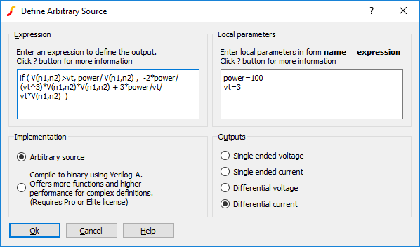
You may specify an equation that defines an output voltage or current in terms of any number of input voltages and currents. Input voltages are specified in the form V(a) or V(a,b) where a and b may be any arbitrary name of your choice. Input currents are specified in the form I(a). On completion, SIMetrix will generate a schematic symbol complete with the input voltages and/or currents that you reference in the equation. There is no need to specify how many input voltages and currents you wish to use. SIMetrix will automatically determine this from the equation.
As well as input voltage and currents, you can also reference the output voltage or current in your equation. A single ended output voltage is accessed using V(out) while a differential output voltage is accessed using V(outp,outn). If you specify an output voltage, you may also access the current flowing through it using I(out).
In the example above, the expression shown - V(vina,vinb)*I(iin) - multiplies a voltage and current together. This could be used to monitor the power in a two terminal device as shown in the following schematic.:
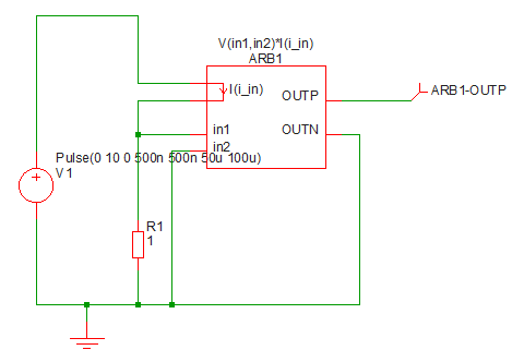
In the above, ARB1 is the device created from the Non-linear Transfer Function menu. ARB1-OUTP will carry a voltage equal to the power dissipation in R1.
In this topic:
Expression
The expression entered defines the output of the device in terms of its inputs. Expressions generally comprise the following elements:
- Circuit variables
- Parameters
- Constants.
- Operators
- Functions
- Look up tables
Circuit Variables
Circuit variables allow the expression to reference input voltages and currents.
Voltages are of the form:
V(node_name1)
V(node_name1, node_name2)
Where node_name1 and node_name2 are input connections.The second form above returns the difference between the voltages on node_name1 and node_name2. The special names out, outp and outn may be used to access the voltage on the output. Use out for the single ended output configuration and outp and/or outn for the differential output configuration.
Currents are of the form:
I(source_name)
Where source_name is the name of an input current. For output voltage configurations, you can use I(out) to access the output current of the device itself. For example
100*I(OUT)
Implements a 100 ohm resistor for a device configured with a differential output voltage.
Parameters
The expression may use any number of parameters. These can be local or global. Local parameters are defined in the Local parameters edit box on the right hand side. Global parameters must defined within the schematic, usually in the F11 window.
To enter local parameters, enter one or more definitions in the form name=expression in the Local parameters edit box. expression may be a constant or an expression referring to other local or global parameters. expression may not contain circuit variables. (E.g. V(in1)). Comment lines may be entered and must start with a '*'.
Built-in Parameters
A number of parameter names are assigned by the simulator. These are:
| Parameter name | Description |
| TIME | Resolves to time for transient analysis. Resolves to 0 otherwise including during the pseudo transient operation point algorithm |
| TEMP | Resolves to current circuit temperature in Celsius |
| HERTZ | Resolves to frequency during AC sweep and zero in other analysis modes |
| PTARAMP | Resolves to value of ramp during pseudo transient operating point algorithm. Otherwise this value resolves to 1. |
Constants
Apart from simple numeric values, arbitrary expressions may also contain the following built-in constants:
| Constant name | Value | Description |
| PI | 3.14159265358979323846 | ???MATH???\pi???MATH??? |
| E | 2.71828182845904523536 | e |
| TRUE | 1.0 | |
| FALSE | 0.0 | |
| ECHARGE | 1.6021918e-19 | Charge on an electron in coulombs |
| BOLTZ | 1.3806226e-23 | Boltzmann's constant |
Operators
These are listed below and are listed in order of precedence. Precedence controls the order of evaluation. So 3*4 + 5*6 = (3*4) + (5*6) = 42 and 3+4*5+6 = 3 + (4*5) + 6 = 29 as '*' has higher precedence than '+'.
| Operator | Description |
| ~ ! - | Digital NOT, Logical NOT, Unary minus |
| ^ or ** | Raise to power. |
| * / | Multiply, divide |
| + - | Plus, minus |
| >= <=, > < | Comparison operators |
| == != or <> | Equal, not equal |
| & | Digital AND (see below) |
| | | Digital OR (see below) |
| && | Logical AND |
| || | Logical OR |
| test ? true_expr : false_expr | Ternary conditional expression (see below) |
Comparison, Equality and Logical Operators
These are Boolean in nature either accepting or returning Boolean values or both. A Boolean value is either TRUE or FALSE. FALSE is defined as equal to zero and TRUE is defined as not equal to zero. So, the comparison and equality operators return 1.0 if the result of the operation is true otherwise they return 0.0.
The arguments to equality operators should always be expressions that can be guaranteed to have an exact value e.g. a Boolean expression or the return value from functions such as SGN. The == operator, for example, will return TRUE only if both arguments are exactly equal. So the following should never be used:
v(n1)==5.5
v(n1) may not ever be exactly 5.0. It may be 5.4999999999 or 5.50000000001 but only by chance will it be 5.5.
These operators are intended to be used with the IF() function described in Ternary Conditional Expression.
Digital Operators
These are the operators '&', '|' and '~'. These are now considered to be obsolete and may not be supported in future versions of SIMetrix. These operators implement logic operations in the analog domain and are continuous in nature.
Ternary Conditional Expression
This is of the form:
test_expression ? true_expression : false_expression
The value returned will be true_expression if test_expression resolves to a non-zero value, otherwise the return value will be false_expression. This is functionally the same as the IF() function described in the functions table below.
Functions
| Function | Description |
| ABS(x) | ???MATH???|x|???MATH??? |
| ACOS(x), ARCCOS(x) | ???MATH???\cos^{-1}(x)???MATH??? |
| ACOSH(x) | ???MATH???\cosh^{-1}(x)???MATH??? |
| ASIN(x), ARCSIN(x) | ???MATH???\sin^{-1}(x)???MATH??? |
| ASINH(x) | ???MATH???\sinh^{-1}(x)???MATH??? |
| ATAN(x), ARCTAN(x) | ???MATH???\tan^{-1}(x)???MATH??? |
| ATAN2(x,y) | ???MATH???\tan^{-1}(x/y)???MATH???. Valid if y=0 |
| ATANH(x) | ???MATH???\tanh^{-1}(x)???MATH??? |
| COS(x) | ???MATH???\cos(x)???MATH??? |
| COSH(x) | ???MATH???\cosh(x)???MATH??? |
| DDT(x) | ???MATH???dx/dt???MATH??? |
| EXP(x) | ???MATH???e^{x}???MATH??? |
| FLOOR(x), INT(x) | Next lowest integer of ???MATH???x???MATH???. |
| GE(x,y[,timetol]) | ???MATH???x>=y???MATH??? See Relational functions. |
| GT(x,y[,timetol]) | ???MATH???x>y???MATH??? See Relational functions. |
| IF(cond, x, y[, maxslew]) | if cond is TRUE ???MATH???result=x???MATH??? else ???MATH???result=y???MATH???. If ???MATH???maxslew>0???MATH??? the rate of change of the result will be slew rate controlled. See IF() Function. |
| IFF(cond, x, y[, maxslew]) | As IF(cond, x, y, maxslew) |
| LE(x,y[,timetol]) | ???MATH???x<=y???MATH??? See Relational functions. |
| LIMIT(x, lo, hi) | if ???MATH???x<lo???MATH??? ???MATH???result=lo???MATH??? else if ???MATH???x>hi???MATH??? ???MATH???result=hi???MATH??? else ???MATH???result=x???MATH??? |
| LIMITS(x, lo, hi, sharp) | As LIMIT but with smoothed corners. The 'sharp' parameter defines the abruptness of the transition. A higher number gives a sharper response. LIMITS gives better convergence than LIMIT. See LIMITS() Function. below |
| LN(x) | ???MATH???\ln(x)???MATH??? If ???MATH???x<10^{-100}???MATH??? ???MATH???result=-230.2585093???MATH??? |
| LNCOSH(x) | ???MATH???\ln(\cosh(x))???MATH??? = ???MATH???\int \tanh(x) dx???MATH??? |
| LOG(x) | ???MATH???ln(x)???MATH??? If ???MATH???x<10^{-100}???MATH??? ???MATH???result=-230.2585093???MATH??? |
| LOG10(x) | ???MATH???log_{10}(x)???MATH???. If ???MATH???x<10^{-100}???MATH??? ???MATH???result=-100???MATH??? |
| LT(x,y[,timetol]) | ???MATH???x<y???MATH??? See Relational functions. |
| MAX(x, y) | Returns larger of ???MATH???x???MATH??? and ???MATH???y???MATH??? |
| MIN(x,y) | Returns smaller of ???MATH???x???MATH??? and ???MATH???y???MATH??? |
| PWR(x,y) | ???MATH???x^y???MATH??? |
| PWRS(x,y) | ???MATH???x>=0???MATH???: ???MATH???x^y???MATH???, ???MATH???x<0???MATH???: ???MATH???-x^y???MATH??? |
| SDT(x) | ???MATH???\int x dt???MATH??? |
| SGN(X) | ???MATH???x>0???MATH???: 1, ???MATH???x<0???MATH???: -1, ???MATH???x=0???MATH???: 0 |
| SIN(x) | ???MATH???\sin(x)???MATH??? |
| SINH(x) | ???MATH???\sinh(x)???MATH??? |
| SQRT(x) | ???MATH???x>=0???MATH???: ???MATH???\sqrt{x}???MATH???, ???MATH???x<0???MATH???: ???MATH???\sqrt{-x}???MATH??? |
| STP(x) | ???MATH???x<=0???MATH???: 0, ???MATH???x>0???MATH???: 1 |
| TABLE(x,xy_pairs) | lookup table. Refer to Lookup tables |
| TABLEX(x,xy_pairs) | Same as TABLE except end points extrapolated. Refer to Lookup tables |
| TAN(x) | ???MATH???\tan(x)???MATH??? |
| TANH(x) | ???MATH???\tanh(x)???MATH??? |
| U(x) | as STP(x) |
| URAMP(x) | ???MATH???x<0???MATH???: 0, ???MATH???x>=0???MATH???: ???MATH???x???MATH??? |
Monte Carlo Distribution Functions
The following functions return a randomly generated value when running a Monte Carlo analysis. They can be used to define component tolerances.
| Name | Distribution | Lot? |
| DISTRIBUTION | User defined distribution | No |
| DISTRIBUTIONL | User defined distribution | Yes |
| UD | Alias for DISTRIBUTION() | No |
| UDL | Alias for DISTRIBUTIONL() | Yes |
| GAUSS | Gaussian | No |
| GAUSSL | Gaussian | Yes |
| GAUSSTRUNC | Truncated Gaussian | No |
| GAUSSTRUNCL | Truncated Gaussian | Yes |
| UNIF | Uniform | No |
| UNIFL | Uniform | Yes |
| WC | Worst case | No |
| WCL | Worst case | Yes |
| GAUSSE | Gaussian logarithmic | No |
| GAUSSEL | Gaussian logarithmic | Yes |
| UNIFE | Uniform logarithmic | No |
| UNIFEL | Uniform logarithmic | Yes |
| WCE | Worst case logarithmic | No |
| WCEL | Worst case logarithmic | Yes |
A full discussion on the use of Monte Carlo distribution functions is given in Simulator Reference Manual/Monte Carlo, Sensitivity and Worst-case/Specifying Tolerances.
IF() Function
IF(condition, true-value, false-value[, max-slew])The result is:
if condition is non-zero, result is true-value, else result is false-value.
If max-slew is present and greater than zero, the result will be slew-rate limited in both positive and negative directions to the value of max-slew.
In some situations, for example if true-value and false-value are constants, the result of this function will be discontinuous when condition changes state. This can lead to non-convergence as there is no lower bound on the time-step. In these cases a max-slew parameter can be included. This will limit the slew rate so providing a controlled transition from the true-value to the false-value and vice-versa.
If the simulator setting .OPTIONS DISCONTINUOUSIFSLEWRATE=max-slew, is provided, SIMetrix will automatically apply a max-slew parameter to all occurrences of the IF() function if both true-value and false-value are constants. This provides a convenient way of resolving convergence issues with third-party models that make extensive use of discontinuous if expressions. Note that the DISCONTINUOUSIFSLEWRATE option is also applied to conditional expressions using the C-style condition ? true-value : false-value syntax.
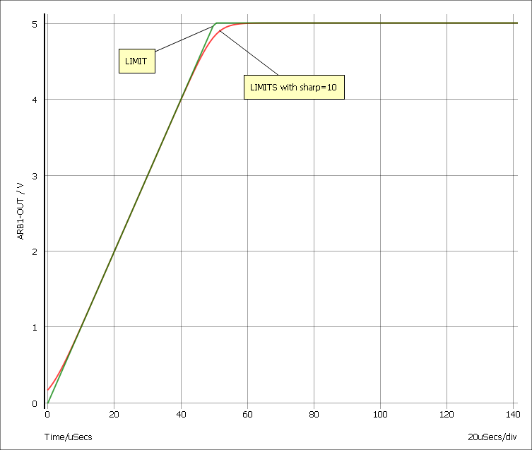
LIMITS() Function
LIMITS(x, low, high, sharp)The LIMITS() function is similar to LIMIT but provides a smooth response at the corners which leads to better convergence behaviour. The behaviour is shown below
The LIMITS function follows this equation:
LIMITS(x, low, high, sharp) = ???MATH???0.5*((\ln(\cosh(v1))-\ln(\cosh(v2)))/v3 +(low+high))???MATH???
- v1 = sharp/(high-low)*(x-low)
- v2 = sharp/(high-low)*(x-high)
- v3 = sharp/(high-low)
Look-up Tables
| Method 1 |
Syntax in form: TABLE[xy_pairs](input_expression).
|
||||
| Method 2 |
Syntax in form: TABLE(input_expression, xy_pairs).
|
||||
| Method 3 |
Syntax in form: TABLEX(input_expression, xy_pairs).
|
Method 1 is more efficient at handling large tables (hundreds of values). However, method 2 is generally more flexible and is the recommended choice for most applications. Method 2 is also compatible with other simulators whereas method 1 is proprietary to SIMetrix.
When designing a table, you should ensure that it covers as wide an input range as possible. While you might only expect a limited voltage (or current) range in your application, the simulator will exercise the inputs to a much wider range while iterating to convergence. In some cases the input range can extend to many orders of magnitude. In many applications, this requirement can be simply achieved by using the TABLEX function which extrapolates to infinity in both directions, However, TABLEX is proprietary to SIMetrix and is not compatible with other simulators.
As an example, consider this simple table designed to implement an approximate diode:
B1 N1 N2 I=TABLE( V(N1,N2), -10,1n, 0,0, 1m,1)
This device will look like a 1m???MATH???\Omega???MATH??? resistor between 0 and 1mV but for voltage drop higher than 1mV it will behave like a 1A current source. It might be that your circuit is not capable of delivering 1A so this may seem acceptable. But the device may converge slowly if voltages higher than 1mV are presented to the device due to the way the simulation algorithms work. Using TABLEX will solve this problem but if wanting something more widely compatible, simply defining a higher input voltage will help a lot. For example:
B1 N1 N2 I=TABLE( V(N1,N2), -10,1n, 0,0, 100, 100000)
For an example see Table Lookup Example
Multi-dimension Look-up Tables
The TABLE() function allows expressions to be used for both X and Y values. The expressions can be other TABLE() functions effectively allowing multi-dimension lookup tables. For example:
B1 N1 N2 I=TABLE(V(TJ), 0,	TABLEX(V(N1,N2), -10,1n, 0,0, 0.5, 1m, 0.6, 1),
+						25, TABLEX(V(N1,N2), -10,2n, 0,0, 0.5, 2m, 0.6, 2),
+						70, TABLEX(V(N1,N2), -10,4n, 0,0, 0.5, 4m, 0.6, 3))
Relational Operators and Functions
The operators '<', '<=', '>' and '>=' are known as relational operators. The result of executing these is a value of either 1.0 or 0.0 depending whether the relation is true. These are often used with the ???MATH???if()???MATH??? function.
The functions, ???MATH???lt(x,y)???MATH???, ???MATH???le(x,y)???MATH???, ???MATH???gt(x,y)???MATH??? and ???MATH???ge(x,y)???MATH??? perform the same task but with an important difference. These functions control the time step so that a time point is performed both before and after the threshold is crossed with a timestep between the two points that is no larger than the value specified by their third argument. If no third argument is provided, a default value is used defined by option setting RELOPTHRESHTIMETOL which itself defaults to 10ns.
The time step control feature of these functions is useful for use in applications such as comparators. For example, suppose a comparator is implemented using an expression such as ???MATH???V(inp) > V(inn)???MATH???. This might be used to trigger activity on the rising edge of an input signal. If the circuit is in an idle state the time steps could be very long, perhaps in the millisecond region. For this example, let's suppose that the timestep is currently 1ms and the ???MATH???V(inp) > V(inn)???MATH??? changes state. This might not be registered until up to 1ms after the threshold is actually crossed. Further the actual delay is random and could therefore introduce quite serious errors maybe even preventing an edge triggered event occurring. This problem is often solved by limiting the maximum time step but in some applications this can slow the simulation time unacceptably.
A better solution is to control the time step so that the threshold is detected accurately. This can be done by instead calling the function ???MATH???lt(V(inp),V(inn),1n)???MATH???. Here the time step will be controlled to an accuracy of 1ns which will solve the problem of slow edges.
The regular operators '<', '<=', '>' and '>=' can also be configured to behave in the same way using another boolean option setting: RELOPTHRESHDETECT. The operators do not have a third argument so these always use the time tolerance defined by RELOPTHRESHTIMETOL. See Simulator Reference Manual/Command Reference/.OPTIONS
Examples
Table Lookup Example
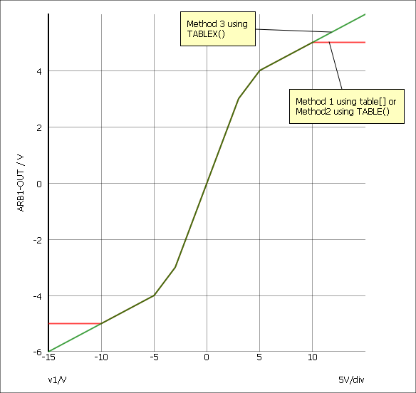
The following arbitrary source definition implements a soft limiting function
table[-10, -5, -5, -4, -4, -3.5, -3, -3, 3, 3, 4, 3.5, 5, 4, 10, 5](v(N1))
TABLE(v(N1), -10, -5, -5, -4, -4, -3.5, -3, -3, 3, 3, 4, 3.5, 5, 4, 10, 5)
TABLEX(v(N1), -10, -5, -5, -4, -4, -3.5, -3, -3, 3, 3, 4, 3.5, 5, 4, 10, 5)
The resulting transfer functions are illustrated in the following picture:
Verilog-A Implementation
If you have SIMetrix Pro or SIMetrix Elite you may select the Compile to binary using Verilog-A option. This will build a definition of the device using the Verilog-A language then compile it to a binary DLL. This process takes place when you run the simulation. The benefit of using Verilog-A is that there is a wider range of functions available and for complex definitions there will also be a performance benefit. Refer to the Verilog-A Manual for details of available functions.
| ◄ Introduction | Laplace Transfer Function ▶ |