Using Expressions
In this topic:
Overview
Expressions consist of arithmetic operators, functions, variables and constants and may be employed in the following locations:
- As device parameters
- As model parameters
- To define a variable (see .PARAM) which can itself be used in an expression.
- As the governing expression used for arbitrary sources.
They have a wide range of uses. For example:
- To define a number of device or model parameters that depend on some common characteristic. This could be a circuit specification such as the cut-off frequency of a filter or maybe a physical characteristic to define a device model.
- To define tolerances used in Monte Carlo analyses.
- Used with an arbitrary source, to define a non-linear device.
Using Expressions for Device Parameters
Device or instance parameters are placed on the device line. For example the length parameter of a MOSFET, L, is a device parameter. A MOSFET line with constant parameters might be:
M1 1 2 3 4 MOS1 L=1u W=2u
L and W could be replaced by expressions. For example:
M1 1 2 3 4 MOS1 L={LL-2*EDGE} W={WW-2*EDGE}
Device parameter expressions must usually be enclosed with either single quotation marks ( ' ) double quotation marks ( " ) or braces ( '{' and '}' ). The expression need not be so enclosed if it consists of a single variable. For example:
.PARAM LL=2u WW=1u
M1 1 2 3 4 MOS1 L=LL W=WW
Using Expressions for Model Parameters
The rules for using expressions for device parameters also apply to model parameters. E.g.
.MODEL N1 NPN IS=is BF={beta*1.3}
Expression Syntax
Expressions generally comprise the following elements:
- Circuit variables
- Parameters
- Constants.
- Operators
- Functions
- Look up tables
Circuit Variables
Circuit variables may only be used in expressions used to define arbitrary sources and to define variables that themselves are accessed only in arbitrary source expressions.
Circuit variables allow an expression to reference voltages and currents in any part of the circuit being simulated.
Voltages are of the form:
V(node_name1)
V(node_name1, node_name2)
Where node_name1 and node_name2 are the name of the node carrying the voltage of interest. The second form above returns the difference between the voltages on node_name1 and node_name2. If using the schematic editor nodenames are normally allocated by the netlist generator. For information on how to display and edit the schematic's node names, refer to Displaying Net and Pin Names.
Currents are of the form:
I(source_name)
Where source_name is the name of a device carrying the current of interest. The controlling device can be any native (i.e. non-subcircuit) device in the circuit. The current used will be the current flowing into its first terminal. The first terminal is the one that is first in the device's netlist entry. Note that if the device is not a voltage source or implemented as a voltage source, the current is sensed by placing a zero-volt voltage source in series with the sensing device. This is done automatically and no user action is required.
It is legal for an expression used in an arbitrary source to reference itself e.g.:
B1 n1 n2 V=100*I(B1)
Implements a 100 ohm resistor.
I(source_name, terminal)where Script Reference Manual/Function Reference/GetDevicePinsexample:
I(Q3,c)
will return the collector current of Q3. There is currently no documentation that lists terminal names for each simulator device type but the names can be obtained from the GetDevicePins script function. Refer to Script Reference Manual/Function Reference/GetDevicePins. Most semiconductor device pins are named with a single letter representing their familiar name: 'c', 'b', 'e', 'd', 'g', 's', 'b' and most two-terminal parts are 'p' and 'n'.
The function names ID, IG, IS, IC, IB and IE may also be used to access drain, gate, source, collector, base and emitter currents respectively. Note, however, that if a user function (defined using .FUNC) of the same name is defined, the user function will take precedence.
Parameters
These are defined using the .PARAM statement. For example:
.PARAM res=100
B1 n1 n2 V=res*I(B1)
Also implements a 100 ohm resistor.
Circuit variables may be used .PARAM statements, for example:
.PARAM VMult = { V(a) * V(b) }
B1 1 2 V = Vmult + V(c)
Parameters that use circuit variables may only be used in places where circuit variables themselves are allowed. So, they can be used in arbitrary sources and they may be used to define the resistance of an Hspice style resistor which allows voltage and current dependence. (See Resistor - Hspice Compatible). They may also of course be used to define further parameters as long as they too comply with the above condition.
Built-in Parameters
A number of parameter names are assigned by the simulator. These are:
| Parameter name | Description | ||||||||||||||
| TIME | Resolves to time for transient analysis. Resolves to 0 otherwise including during the pseudo transient operation point algorithm. Note that this may only be used in an arbitrary source expression | ||||||||||||||
| TEMP | Resolves to current circuit temperature in Celsius | ||||||||||||||
| HERTZ | Resolves to frequency during AC sweep and zero in other analysis modes | ||||||||||||||
| PTARAMP | Resolves to value of ramp during pseudo transient operating point algorithm if used in arbitrary source expression. Otherwise this value resolves to 1 | ||||||||||||||
| STARTUPRAMP | Resolves to transient startup ramp value when a "startup" specification is provided. During a startup phase this will have a value that rises linearly from 0.0 at t=0 to 1.0 when t reaches the startup time | ||||||||||||||
| ANALYSIS |
Resolves to an integer value according to the analysis being performed.
|
Constants
Apart from simple numeric values, arbitrary expressions may also contain the following built-in constants:
| Constant name | Value | Description |
| PI | 3.14159265358979323846 | ???MATH???\pi???MATH??? |
| E | 2.71828182845904523536 | e |
| TRUE | 1.0 | |
| FALSE | 0.0 | |
| ECHARGE | 1.6021918e-19 | Charge on an electron in coulombs |
| BOLTZ | 1.3806226e-23 | Boltzmann's constant |
B1 n1 n2 V = V(n3, n3) * { global:amp_gain }
amp_gain could be defined in a script using the LET command. E.g. "Let global:amp_gain = 100"
Operators
These are listed below and are listed in order of precedence. Precedence controls the order of evaluation. So 3*4 + 5*6 = (3*4) + (5*6) = 42 and 3+4*5+6 = 3 + (4*5) + 6 = 29 as '*' has higher precedence than '+'.
| Operator | Description |
| ~ ! - | Digital NOT, Logical NOT, Unary minus |
| ^ or ** | Raise to power. |
| *, / | Multiply, divide |
| +, - | Plus, minus |
| >=, <=, > < | Comparison operators |
| ==, != or <> | Equal, not equal |
| & | Digital AND (see below) |
| | | Digital OR (see below) |
| && | Logical AND |
| ^^ | Exclusive OR |
| || | Logical OR |
| test ? true_expr : false_expr | Ternary conditional expression (see below) |
Comparison, Equality and Logical Operators
These are Boolean in nature either accepting or returning Boolean values or both. A Boolean value is either TRUE or FALSE. FALSE is defined as equal to zero and TRUE is defined as not equal to zero. So, the comparison and equality operators return 1.0 if the result of the operation is true otherwise they return 0.0.
The arguments to equality operators should always be expressions that can be guaranteed to have an exact value e.g. a Boolean expression or the return value from functions such as SGN. The == operator, for example, will return TRUE only if both arguments are exactly equal. So the following should never be used:
v(n1)==5.0
v(n1) may not ever be exactly 5.0. It may be 4.9999999999 or 5.00000000001 but only by chance will it be 5.0.
These operators are intended to be used with the IF() function described in Ternary Conditional Expression.
Digital Operators
These are now considered obsolete and should not be used in new model designs. They may be removed from future versions of SIMetrix.
These are the operators '&', '|' and '~'. These were introduced in old SIMetrix version as a simple means of implementing digital gates in the analog domain. Their function has largely been superseded by gates in the event driven simulator.
Ternary Conditional Expression
This is of the form:
test_expression ? true_expression : false_expression
The value returned will be true_expression if test_expression resolves to a non-zero value, otherwise the return value will be false_expression. This is functionally the same as the IF() function described in the functions table below.
Functions
| Function | Description |
| ABS(x) | ???MATH???|x|???MATH??? |
| ACOS(x), ARCCOS(x) | ???MATH???cos^{-1}(x)???MATH??? |
| ACOSH(x) | ???MATH???cosh^{-1}(x)???MATH??? |
| ASIN(x), ARCSIN(x) | ???MATH???sin^{-1}(x)???MATH??? |
| ASINH(x) | ???MATH???sinh^{-1}(x)???MATH??? |
| ATAN(x), ARCTAN(x) | ???MATH???tan^{-1}(x)???MATH??? |
| ATAN2(x,y) | ???MATH???tan^{-1}(x/y)???MATH???. Valid if y=0 |
| ATANH(x) | ???MATH???tanh^{-1}(x)???MATH??? |
| COS(x) | ???MATH???cos(x)???MATH??? |
| COSH(x) | ???MATH???cosh(x)???MATH??? |
| DELAY(x, delay, [max_delay]) | Delays ???MATH???x???MATH??? by ???MATH???delay???MATH???. ???MATH???max_delay???MATH??? if provided sets a maximum value for ???MATH???delay???MATH???. ???MATH???delay???MATH??? must be a constant unless a value for ???MATH???max_delay???MATH??? is provided. |
| DDT(x) | ???MATH???dx/dt???MATH??? |
| EXP(x) | ???MATH???e^{x}???MATH??? |
| FLOOR(x), INT(x) | Next lowest integer of ???MATH???x???MATH???. |
| GE(x,y[,timetol]) | ???MATH???x>=y???MATH??? See Relational functions. |
| GT(x,y[,timetol]) | ???MATH???x>y???MATH??? See Relational functions. |
| IF(cond, x, y[, maxslew]) | if cond is TRUE ???MATH???result=x???MATH??? else ???MATH???result=y???MATH???. If ???MATH???maxslew>0???MATH??? the rate of change of the result will be slew rate controlled. See IF() Function. |
| IFF(cond, x, y[, maxslew]) | As IF(cond, x, y, maxslew) |
| LE(x,y[,timetol]) | ???MATH???x<=y???MATH??? See Relational functions. |
| LIMIT(x, lo, hi) | if ???MATH???x<lo???MATH??? ???MATH???result=lo???MATH??? else if ???MATH???x>hi???MATH??? ???MATH???result=hi???MATH??? else ???MATH???result=x???MATH??? |
| LIMITS(x, lo, hi, sharp) | As LIMIT but with smoothed corners. The 'sharp' parameter defines the abruptness of the transition. A higher number gives a sharper response. LIMITS gives better convergence than LIMIT. See LIMITS() Function. below |
| LN(x) | ???MATH???ln(x)???MATH??? If ???MATH???x<10^{-100}???MATH??? ???MATH???result=-230.2585093???MATH??? |
| LNCOSH(x) | ???MATH???ln(cosh(x))???MATH??? = ???MATH???\int tanh(x) dx???MATH??? |
| LOG(x) | ???MATH???ln(x)???MATH??? If ???MATH???x<10^{-100}???MATH??? ???MATH???result=-230.2585093???MATH??? See note |
| LOG10(x) | ???MATH???log_{10}(x)???MATH???. If ???MATH???x<10^{-100}???MATH??? ???MATH???result=-100???MATH??? |
| LT(x,y[,timetol]) | ???MATH???x<y???MATH??? See Relational functions. |
| MAX(x, y) | Returns larger of ???MATH???x???MATH??? and ???MATH???y???MATH??? |
| MIN(x,y) | Returns smaller of ???MATH???x???MATH??? and ???MATH???y???MATH??? |
| PWR(x,y) | ???MATH???x^y???MATH??? |
| PWRS(x,y) | ???MATH???x>=0???MATH???: ???MATH???x^y???MATH???, ???MATH???x<0???MATH???: ???MATH???-x^y???MATH??? |
| SDT(x) | ???MATH???\int x dt???MATH??? |
| SGN(X) | ???MATH???x>0???MATH???: 1, ???MATH???x<0???MATH???: -1, ???MATH???x=0???MATH???: 0 |
| SIN(x) | ???MATH???sin(x)???MATH??? |
| SINH(x) | ???MATH???sinh(x)???MATH??? |
| SQRT(x) | ???MATH???x>=0???MATH???: ???MATH???\sqrt{x}???MATH???, ???MATH???x<0???MATH???: ???MATH???\sqrt{-x}???MATH??? |
| STP(x) | ???MATH???x<=0???MATH???: 0, ???MATH???x>0???MATH???: 1 |
| TABLE(x,xy_pairs) | lookup table. Refer to Lookup tables |
| TABLEX(x,xy_pairs) | Same as TABLE except end points extrapolated. Refer to Lookup tables |
| TAN(x) | ???MATH???tan(x)???MATH??? |
| TANH(x) | ???MATH???tanh(x)???MATH??? |
| U(x) | as STP(x) |
| URAMP(x) | ???MATH???x<0???MATH???: 0, ???MATH???x>=0???MATH???: ???MATH???x???MATH??? |
The log() Function
In versions 9.1 and earlier the log() function means log to the base 10 in native SIMetrix expressions. From 9.2 this changed to log to the base e in order to be compatible with other simulators and publicly available models.
If compatibility with older SIMetrix versions is required, an option setting can be used to revert to log to base 10. Add this line to the netlist:
.OPTIONS logFunctionBaseE=0
Note that the above affects the use of log() in native arbitrary source expressions and .PARAM statements. A native arbitrary source is one defined using the 'B' device as follows:
Bxxx n1 n2 v|i|q|flux = expression
See Arbitrary Source for further details.
Arbitrary sources implemented using PSpice ABM syntax are also recognised by SIMetrix and, as PSpice interprets log() as log to base e, SIMetrix will do so too when used in a PSpice ABM expression regardless of the logFunctionBaseE option setting. For example:
E1 n1 n2 VALUE = {log(1+exp(V(n3,n4)))}
In the above, log is interpreted as log to base e even if the logFunctionBaseE option setting above is set to 0.
To avoid any confusion, we recommend avoid using log(). For log to base 10 use log10() and for log to base e use ln().
Monte Carlo Distribution Functions
To specify Monte Carlo tolerance for a model parameter, use an expression containing one of the following functions:
| Name | Distribution | Lot? |
| DISTRIBUTION2 | User defined distribution | No |
| DISTRIBUTION2L | User defined distribution | Yes |
| UD2 | Alias for DISTRIBUTION2() | No |
| UD2L | Alias for DISTRIBUTION2L() | Yes |
| GAUSS | Gaussian | No |
| GAUSSL | Gaussian | Yes |
| GAUSSTRUNC | Truncated Gaussian | No |
| GAUSSTRUNCL | Truncated Gaussian | Yes |
| UNIF | Uniform | No |
| UNIFL | Uniform | Yes |
| UNIF2 | Uniform | No |
| UNIFL2 | Uniform | Yes |
| WC | Worst case | No |
| WCL | Worst case | Yes |
| WC2 | Worst case | No |
| WCL2 | Worst case | Yes |
| GAUSSE | Gaussian logarithmic | No |
| GAUSSEL | Gaussian logarithmic | Yes |
| UNIFE | Uniform logarithmic | No |
| UNIFEL | Uniform logarithmic | Yes |
| WCE | Worst case logarithmic | No |
| WCEL | Worst case logarithmic | Yes |
IF() Function
IF(condition, true-value, false-value[, max-slew])The result is:
if condition is non-zero, result is true-value, else result is false-value.
If max-slew is present and greater than zero, the result will be slew-rate limited in both positive and negative directions to the value of max-slew.
In some situations, for example if true-value and false-value are constants, the result of this function will be discontinuous when condition changes state. This can lead to non-convergence as there is no lower bound on the time-step. In these cases a max-slew parameter can be included. This will limit the slew rate so providing a controlled transition from the true-value to the false-value and vice-versa.
If the option setting DISCONTINUOUSIFSLEWRATE is non-zero, SIMetrix will automatically apply a max-slew parameter to all occurrences of the IF() function if both true-value and false-value are constants. This provides a convenient way of resolving convergence issues with third-party models that make extensive use of discontinuous if expressions. Note that the DISCONTINUOUSIFSLEWRATE option is also applied to conditional expressions using the C-style condition ? true-value : false-value syntax.
LIMITS() Function
LIMITS(x, low, high, sharp)The LIMITS() function is similar to LIMIT but provides a smooth response at the corners which leads to better convergence behaviour. The behaviour is shown below
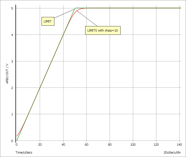
The LIMITS function follows this equation:
LIMITS(x, low, high, sharp) = 0.5*((ln(cosh(v1))-ln(cosh(v2)))/v3 +(low+high))
- v1 = sharp/(high-low)*(x-low)
- v2 = sharp/(high-low)*(x-high)
- v3 = sharp/(high-low)
Look-up Tables
| Method 1 |
Syntax in form: TABLE[xy_pairs](input_expression).
|
||||
| Method 2 |
Syntax in form: TABLE(input_expression, xy_pairs).
|
||||
| Method 3 |
Syntax in form: TABLEX(input_expression, xy_pairs).
|
Method 1 is more efficient at handling large tables (hundreds of values). However, method 2 is generally more flexible and is the recommended choice for most applications. Method 2 is also compatible with other simulators whereas method 1 is proprietary to SIMetrix.
When designing a table, you should ensure that it covers as wide an input range as possible. While you might only expect a limited voltage (or current) range in your application, the simulator will exercise the inputs to a much wider range while iterating to convergence. In some cases the input range can extend to many orders of magnitude. In many applications, this requirement can be simply achieved by using the TABLEX function which extrapolates to infinity in both directions, However, TABLEX is proprietary to SIMetrix and is not compatible with other simulators.
As an example, consider this simple table designed to implement an approximate diode:
B1 N1 N2 I=TABLE( V(N1,N2), -10,1n, 0,0, 1m,1)
This device will look like a 1m???MATH???\Omega???MATH??? resistor between 0 and 1mV but for voltage drop higher than 1mV it will behave like a 1A current source. It might be that your circuit is not capable of delivering 1A so this may seem acceptable. But the device may converge slowly if voltages higher than 1mV are presented to the device due to the way the simulation algorithms work. Using TABLEX will solve this problem but if wanting something more widely compatible, simply defining a higher input voltage will help a lot. For example:
B1 N1 N2 I=TABLE( V(N1,N2), -10,1n, 0,0, 100, 100000)
For an example see Table Lookup Example
Multi-dimension Look-up Tables
The TABLE() function allows expressions to be used for both X and Y values. The expressions can be other TABLE() functions effectively allowing multi-dimension lookup tables. For example:
B1 N1 N2 I=TABLE(V(TJ), 0,	TABLEX(V(N1,N2), -10,1n, 0,0, 0.5, 1m, 0.6, 1),
+						25, TABLEX(V(N1,N2), -10,2n, 0,0, 0.5, 2m, 0.6, 2),
+						70, TABLEX(V(N1,N2), -10,4n, 0,0, 0.5, 4m, 0.6, 3))
Relational Operators and Functions
The operators '<', '<=', '>' and '>=' are known as relational operators. The result of executing these is a value of either 1.0 or 0.0 depending whether the relation is true. These are often used with the ???MATH???if()???MATH??? function.
The functions, ???MATH???lt(x,y)???MATH???, ???MATH???le(x,y)???MATH???, ???MATH???gt(x,y)???MATH??? and ???MATH???ge(x,y)???MATH??? perform the same task but with an important difference. These functions control the time step so that a time point is performed both before and after the threshold is crossed with a timestep between the two points that is no larger than the value specified by their third argument. If no third argument is provided, a default value is used defined by option setting RELOPTHRESHTIMETOL which itself defaults to 10ns.
The time step control feature of these functions is useful for use in applications such as comparators. For example, suppose a comparator is implemented using an expression such as ???MATH???V(inp) > V(inn)???MATH???. This might be used to trigger activity on the rising edge of an input signal. If the circuit is in an idle state the time steps could be very long, perhaps in the millisecond region. For this example, let's suppose that the timestep is currently 1ms and the ???MATH???V(inp) > V(inn)???MATH??? changes state. This might not be registered until up to 1ms after the threshold is actually crossed. Further the actual delay is random and could therefore introduce quite serious errors maybe even preventing an edge triggered event occurring. This problem is often solved by limiting the maximum time step but in some applications this can slow the simulation time unacceptably.
A better solution is to control the time step so that the threshold is detected accurately. This can be done by instead calling the function ???MATH???lt(V(inp),V(inn),1n)???MATH???. Here the time step will be controlled to an accuracy of 1ns which will solve the problem of slow edges.
The regular operators '<', '<=', '>' and '>=' can also be configured to behave in the same way using another boolean option setting: RELOPTHRESHDETECT. The operators do not have a third argument so these always use the time tolerance defined by RELOPTHRESHTIMETOL. See .OPTIONS
Examples
Table Lookup Example
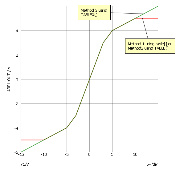
The following arbitrary source definition implements a soft limiting function
B1 n2 n3 V=table[-10, -5, -5, -4, -4, -3.5, -3, -3, 3, 3, 4,
+ 3.5, 5, 4, 10, 5](v(N1))
B1 n2 n3 V=TABLE(v(N1), -10, -5, -5, -4, -4, -3.5, -3, -3, 3, 3, 4,
+ 3.5, 5, 4, 10, 5)
B1 n2 n3 V=TABLEX(v(N1), -10, -5, -5, -4, -4, -3.5, -3, -3, 3, 3, 4,
+ 3.5, 5, 4, 10, 5)
The resulting transfer functions are illustrated in the following picture:
Parameter Example
It is possible to assign expressions to component values which are evaluated when the circuit is simulated. This has a number of uses. For example you might have a filter design for which several component values affect the roll off frequency. Rather than recalculate and change each component every time you wish to change the roll of frequency it is possible to enter the formula for the component's value in terms of this frequency.
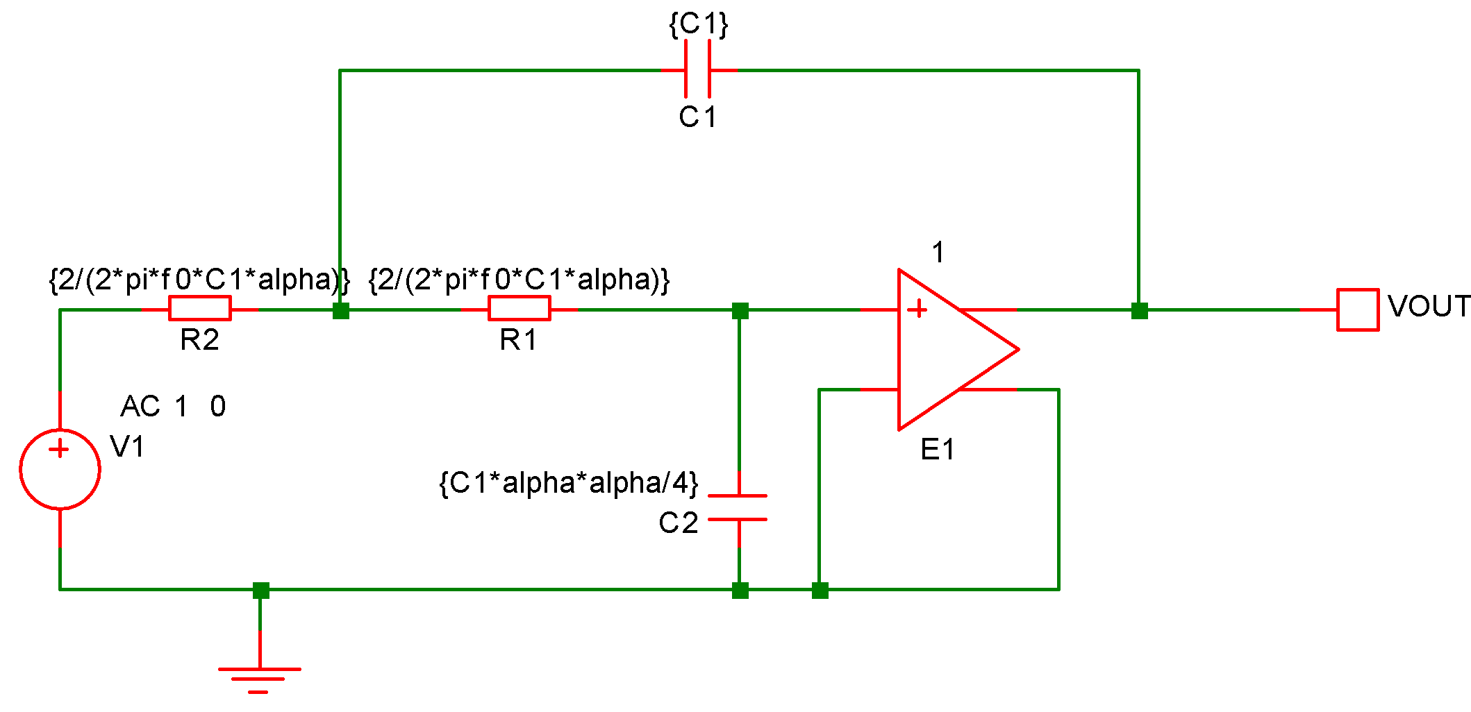
The above circuit is that of a two pole low-pass filter. C1 is fixed and R1=R2. The design equations are:
R1=R2=2/(2*pi*f0*C1*alpha)
C2=C1*alpha*alpha/4
where f0 is the cut off frequency and alpha is the damping factor.
The complete netlist for the above circuit is:
V1 V1_P 0 AC 1 0
C2 0 R1_P {C1*alpha*alpha/4}
C1 VOUT R1_N {C1}
E1 VOUT 0 R1_P 0 1
R1 R1_P R1_N {2/(2*pi*f0*C1*alpha)}
R2 R1_N V1_P {2/(2*pi*f0*C1*alpha)}
Before running the above circuit you must assign values to the variables. This can be done by one of three methods:
- With the .PARAM statement placed in the netlist.
- With Let command from the command line or from a script. (If using a script you must prefix the parameter names with global:)
- By sweeping the value with using parameter mode of a swept analysis (see General Sweep Specification) or multi-step analysis (see Multi Step Analyses).
Suppose we wish a 1kHz roll off for the above filter.
Using the .PARAM statement, add these lines to the netlist
.PARAM f0 1k
.PARAM alpha 1
.PARAM C1 10n
Using the Let command, you would type:
Let f0=1k
Let alpha=1
Let C1=10n
Let alpha=0.8
then re-run the simulator.
To execute the Let commands from within a script, prefix the parameter names with global:. E.g. "Let global:f0=1k"
In many cases the .PARAM approach is more convenient as the values can be stored with the schematic.
Optimisation
Overview
An optimisation algorithm may be enabled for expressions used to define arbitrary sources and any expression containing a swept parameter. This can improve performance if a large number of such expressions are present in a design.
The optimiser dramatically improves the simulation performance of the power device models developed by Infineon. See Optimiser Performance.
Note that the optimiser referred to here is an algorithm that manipulates expressions found in arbitrary sources to make them evaluate more efficiently. This is not to be confused with the circuit optimiser described here
Why is it Needed?
The simulator's core algorithms use the Newton-Raphson iteration method to solve non-linear equations. This method requires the differential of each equation to be calculated and for arbitrary sources, this differentiation is performed symbolically. So as well as calculating the user supplied expression, the simulator must also evaluate the expression's differential with respect to each dependent variable. These differential expressions nearly always have some sub-expressions in common with sub-expressions in the main equation and other differentials. Calculation speed can be improved by arranging to evaluate these sub-expressions only once. This is the main task performed by the optimiser. However, it also eliminates factors found on both the numerator and denominator of an expression as well as collecting constants together wherever possible.
Using the Optimiser
The optimiser is automatically enabled and no action is required to make use of it. If desired, it can be disabled using:
.OPTIONS optimise=0
Optimiser Performance
The optimisation algorithm was added to SIMetrix primarily initially to improve the performance of some publicly available power device models from Infineon. These models make extensive use of arbitrary sources and many expressions are defined using .FUNC. Since its original development, many more device manufacturers have developed models using the same method and these also benefit from the performance enhancement.
The performance improvement gained for these model is in some cases dramatic. For example a simple switching PSU circuit using a SGP02N60 IGBT ran around 5 times faster with the optimiser enabled and there are other devices that show an even bigger improvement.
Accuracy
The optimiser simply changes the efficiency of evaluation and doesn't change the calculation being performed in any way. However, performing a calculation in a different order can alter the least significant digits in the final result. In some simulations, these tiny changes can result in much larger changes in circuit solution. So, you may find that switching the optimiser on and off may change the results slightly.
| ◄ Using XSPICE Devices | Subcircuits ▶ |