Piecewise Linear Modeling
SIMPLIS achieves its speed by modeling devices using a series of Piecewise Linear (PWL) straight-line segments rather than by using the SPICE technique of solving nonlinearities such as exponential expressions.
Piecewise Linear Resistors
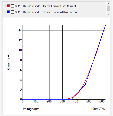
Here we compare a Spice model (in red) of the current vs. voltage characteristic of the body diode of the Si4410DY NMOS Q1 with a SIMPLIS PWL model (in blue). SIMPLIS uses a PWL Resistor to model this diode characteristic.
Piecewise Linear Capacitors
A good example of a SIMPLIS PWL capacitor application is the four-segment PWL capacitor used to model a diode junction capacitance as shown below. The SIMPLIS PWL capacitance parameter values were determined by an automated SIMPLIS model parameter extraction routine.
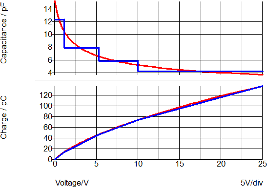
These curves show both the capacitance and charge versus the reverse voltage for the diode in this example. On the upper graph, the red curve shows the continuous capacitance change of the SPICE model with reverse voltage. The blue curve shows the SIMPLIS step-wise constant capacitance versus the reverse voltage curve.
The lower graph shows the charge versus reverse voltage with the SPICE model in red and the SIMPLIS model in blue. Although the error between points on the capacitance curve appears to be large at certain voltage values, the error between the two charge curves is quite small. In most switch-mode applications, the total capacitive charge versus voltage characteristic is the dominant factor in determining device transitions from a conducting state to a blocking state and vice-versa. Consequently, PWL capacitors can be used to accurately represent junction capacitances in switch-mode power conversion applications.
Accuracy of Piecewise Linear Modeling
Because PWL modeling is a bit unfamiliar to many first-time SIMPLIS users, it is not uncommon to confuse piecewise linear modeling with the creation of idealized models. And while PWL modeling easily supports the creation of idealized models, it can also be the most accurate practical method of modeling the switching losses in DC-DC and AC-DC power supplies. In the next example, we modify the model level of Q1 in our buck converter from model level 0 (an instantaneous switch with an ON resistance and an OFF resistance) to model level 2, which models the nonlinear Gate-to-Drain and Drain-to-Source capacitance on the MOSFET as well as the active region of the device. In this fashion, we can model the switching transitions of a MOSFET with a high degree of accuracy.
In this next schematic, we modify the model level of the MOSFET Q1 from model level 0 to model level 2.
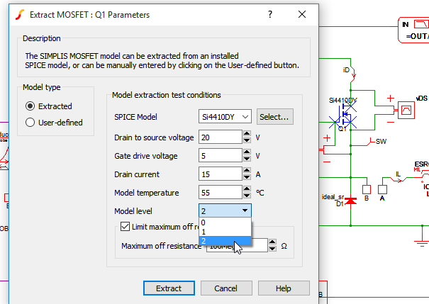
Click to download a Buck Converter Schematic where the MOSFET model of Q1 has been changed to level 2.
Run the default simulation. It is set up to run a Periodic Operating Point (POP) analysis to find the steady-state of the system. In the waveform viewer click on the tab labeled Power(Q1). This tab plots the Gate-to-Source voltage vGS, the Drain-to-Source voltage vDS, and the Drain current iD waveforms of Q1. We also see plotted the Gate current iG as well as the instantaneous power dissipated in Q1. Zoom in on one set of ON-OFF transitions as shown here.
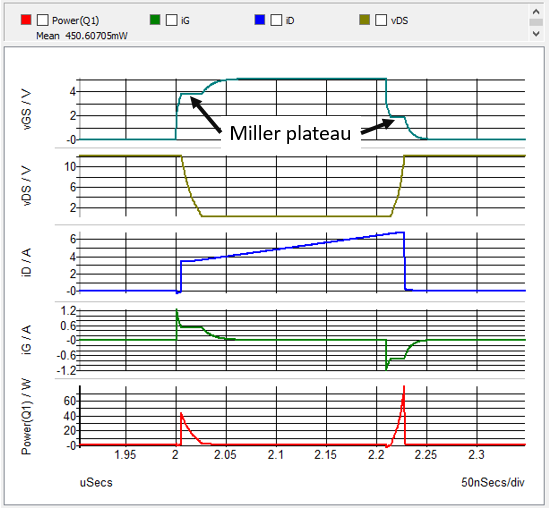
We can see the Miller effect evident in the finite transitions of these waveforms, including the Miller plateau on the vGS waveform during both the turn-ON and turn-OFF transitions.
The following link is a good executive summary of the accuracy of PWL models in SIMPLIS.
In this summary, SIMPLIS simulation results are compared with lab measurements for:
- a step load change at the output of a synchronous buck converter,
- the detailed switching waveforms of a power MOSFET, and
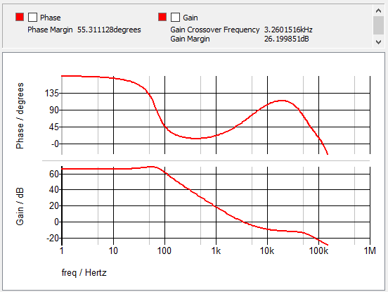
- the Bode plot of a variable frequency flyback DC-DC converter.
While achieving very accurate results, by employing PWL device models in this way, SIMPLIS can characterize a complex nonlinear system as a cyclical sequence of piecewise linear circuit topologies. This method of handling power-supply system nonlinearities is typically 10 to 50 times faster than Spice and avoids the convergence issues inherent with Spice type approaches. Not only does this method generate an accurate representation of the closed-loop performance of a typical switching power system, but we also see that SIMPLIS can accurately predict the detailed switching transitions of those semiconductor devices functioning as high-frequency switches.
Next, we explore how we can exploit the accuracy and speed of SIMPLIS to model much more complex topologies than would be feasible with SPICE-based approaches. The next circuit example of a single-switch dual-output forward converter with coupled output inductors demonstrates this point.
Download the circuit by clicking on this link.
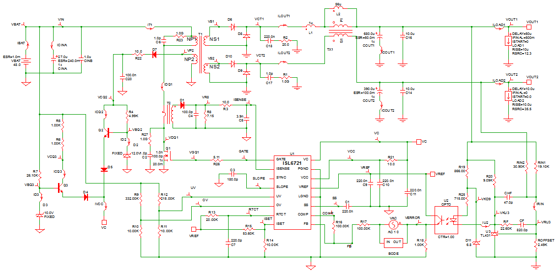
Run the simulation by pressing the F9 key or clicking on the Run Schematic icon. This schematic is set up to do a POP analysis, followed by a Bode Plot and then a step load transient on the main output VOUT1.
Note that the AC analysis is performed on the full nonlinear time-domain switching circuit. There is no need to derive an average model to perform the AC analysis.
The speed with which SIMPLIS simulates this large and quite complex schematic demonstrates one aspect of how SIMPLIS makes it practical to do in-depth design verification before the first hardware models of a design are built.
Another way that SIMPLIS speeds up the simulation process is with the POP analysis.
What SIMPLIS POP Does
The SIMPLIS Periodic Operating Point (POP) analysis excels at finding the steady-state ON-OFF limit cycle of a stable periodic switching system. The SIMPLIS POP analysis can accomplish this much faster, more accurately and far more repeatably than by running a long time domain transient simulation. The high accuracy of the POP analysis enables practical loss analysis and also enables small signal AC analysis based on the full nonlinear time-domain simulation model. Useful loss analysis and AC analysis require that the system be in periodic steady state in order to achieve accurate and repeatable results. Because of its uniqueness to SIMPLIS, POP analysis is one of the more challenging, but also more rewarding aspects of SIMPLIS to master.
The Dual Output Single Switch Forward Converter Schematic is an excellent example of how SIMPLIS can find the steady-state operating point of a complex power supply system very quickly and accurately.
Understanding how the SIMPLIS POP analysis and the POP algorithm work is critical to receiving the maximum benefit from the SIMPLIS simulation capability.
To find steady state, POP simulates the system in the time domain by performing these tasks:
- Takes a snapshot of every capacitor voltage and every inductor current at the beginning of each switching cycle.
- Simulates the system for an additional switching cycle, and then takes another snapshot of the system at the beginning of the next switching cycle.
- Takes the difference of each capacitor voltage and each inductor current between these two snapshots, seeking to drive each difference to zero.
In practice, once POP has found the steady state of a switching system, the largest difference between two successive snapshot values for capacitor voltage or inductor current is in the range of 1.0E-10 % to 1.0E-13 %. These are miniscule errors compared to a typical RELTOL in SPICE of 1.0E-3.
In a system with a reasonable set of initial conditions, the SIMPLIS POP algorithm iteratively seeks the following conditions to arrive at a steady state.
- For each capacitor voltage, the voltage difference in snapshot values from cycle to cycle is nearly zero.
- For each inductor current, the difference in current snapshot values from cycle to cycle is nearly zero.
This SIMPLIS POP algorithm works best in finding the steady-state operating point of switching time-sampled systems such as the following:
- Switching power supplies
- Phase-locked loops
- Class D amplifiers
- Switched capacitor filters
Many of these systems use a feedback loop for control. If the system with its feedback loop is unstable and has no steady-state operating point, then the POP analysis will not be successful. As long as this feedback system is stable, the POP analysis can be successful.
Why SIMPLIS POP Matters
In real life, when you characterize a switching system such as a switching power supply, more than 95% of the measurements begin with the system in steady state operation. The SIMPLIS POP analysis quickly drives a switching circuit into a steady state. Once the system reaches steady state, the system can be purturbed and the resulting system response can be measured.
In the overwhelming majority of system measurements, the reference point for the measurement is an initial steady-state periodic operating point. Since in a typical design project, the designer runs several thousand simulations, being able to reduce the amount of CPU time required to get the system into steady state pays off in time saved for the engineer. If the time to reach steady state can be reduced from 10 minutes to 10 seconds, the time savings runs into hundreds of hours over the life of a project.
Because SIMPLIS can run so many simulations in a relatively short period of time, the SIMPLIS POP analysis makes serious simulation analysis feasible for switching power supply systems. Without POP, only a cursory set of simulation analyses can be run in the practical time allowed. POP, however, makes possible exhaustive system performance characterization during the design process. As a result, the majority of design errors can be detected very early in the design process. Detecting errors before the design has been committed to hardware is the best time in the design process to detect design errors because then they are least expensive in time and money to correct.
Because of the speed and accuracy with which the piecewise linear SIMPLIS POP analysis can find steady state means, SIMPLIS AC analysis is possible based on the following two-step process:
- While performing a time-domain transient simulation with the system in steady state, an extremely small AC signal injected into the system assures that nothing disturbs the system in such a way that inadvertently saturates any device in the signal path.
- The system response to the injected signal is then measured again in the time domain. The accuracy of SIMPLIS is so high, that even with a very small injected AC signal, this system response can be measured with an extremely good signal-to-noise ratio.
Next Steps
- Next, we suggest that you go through the SIMPLIS Tutorial to get an excellent hands-on introduction to creating schematics and running simulations in SIMPLIS.
- After going through the SIMPLIS Tutorial you will be ready to make good use of a free SIMetrix/SIMPLIS Evaluation License. This Evaluation License will provide you with access to a time-limited license with the full capabilities of SIMetrix/SIMPLIS, without the circuit size limitations of SIMetrix/SIMPLIS Elements which you may download for free.